Scientific Investigation, Part II

The Power of Science

Science is a process, not just a body of knowledge. In a broad sense, everyone is a scientist. A small child learns about the forces of gravity and friction by experimenting with toys. Advancements in science occur by making a hypothesis, designing experiments to test them, collecting data, drawing conclusions, and revising the hypothesis based on accumulated data is science. The scientific method is based on a clear set of logical steps that lead to a conclusion based on actual data.

Science is a process for discovery, and it does not end once a question is answered. Each discovery leads to new questions. Each advance opens up new fields of research. Today’s frontiers in science are built on the hypotheses and theories that directed past research. A sampling of these frontiers includes:

• nanotechnology—builds new materials at both the atomic and molecular level
• biotechnology—engineers on the scale of a living cell; includes genetic engineering of DNA molecules
• agro-ecology—combines the study of natural ecosystems and social sciences to build sustainable agriculture
• information technology—develops computer systems and techniques to manage data more efficiency
• climate modeling—uses computers to build models of the complex systems of Earth’s atmosphere and oceans

Measuring Up to Science

Although mathematics is a branch of science, it is also a key tool for nearly all scientific investigations. Because conclusions rely on reproducible data, most scientific investigations involve measurement of one or more physical quantities. Some attributes that can be measured include length, mass, volume, time, temperature, and number of particles. Every measurement has two components: a unit that is associated with a physical quantity, such as length or mass, and the measured number of units. Both parts of a measurement must be included. For example, a length of 2 is not a meaningful measurement, while 2 millimeters, 2 kilometers, 2 inches, and 2 light-years are all meaningful measurements.

Over the course of history, people have developed many different systems of measurement. For example, one distance can be expressed as 2.00 meters, 6.56 feet, 0.4 rods, or 0.00124 mile. Sharing data and experimental results is much easier, however, if everyone uses the same units.

Scientists around the world have agreed to use a metric system of measurement, based on powers of ten, known as the International System of Units (SI). The system uses fundamental units for length, time, mass, temperature, electric current, amount of a substance, and luminosity.

Units that are larger or smaller than the base unit are designated in SI by prefixes that indicate their value in different powers of ten. The table below shows the SI prefixes and their values. Note that the base unit of mass (kg) is defined as 1000 grams.

Other derived units, such as those for density, speed, and power are combinations of the fundamental units of the SI system. The table below lists a number of derived units and their relationship to the SI base units.

Measured values can be treated just as regular numbers, added, or subtracted, but only if their units are the same. How do you work with measurements that use different units—for example (500 m + 2.3 km) or (6 ft – 1 m)? A conversion factor is a ratio of equivalent values that expresses a single quantity in two different units. For example, let’s look at 1 km = 1,000 m.

(500 m) (1 km/1000 m) = 0.5 km

After making this conversion, you can add the first example above

500 m + 2.3 km = 0.5 km + 2.3 km = 2.8 km

Note that the 2.3 km can alternatively be converted to 2,300 m, yielding a sum of 2,800 m.

Using units incorrectly can have drastic effects on results of an experiment. In 1999, NASA sent a probe, the Mars Climate Orbiter, to investigate the Martian atmosphere. After the rockets that were supposed to place the probe into an orbit around Mars fired, the probe was lost, apparently crashing on the surface. An investigation revealed that two teams of scientists and engineers had worked on the calculations needed to time the firing of the rockets. One team had used SI units and the other had used English units (feet and pounds). Oops.

Below are a number of sample conversion tables that are fairly straight forward, but not exhaustive. Take a little time to reacquaint yourself with the different units and understand the different and relative values (e.g., you should know that a kilogram is roughly twice as much a pound). Please note that we have not included all possible conversions.

In addition to measurements of dimensions and time, many scientific investigations measure temperature. How should you dress if the weather report calls for a high temperature of 35°? That depends. If the temperature is 35°F, you will want to bundle up; if it is 35°C, light clothes are in order. If the temperature is 35K, then you are probably on the Moon, not Earth. These values correspond to the three main temperature scales used in science. The illustration shows several equivalent temperatures, including the melting and boiling points of water on the Fahrenheit, Celsius, and Kelvin scales. A third point, absolute zero, is the theoretical coldest possible temperature. Absolute zero is the starting point of the Kelvin scale.

Although the Fahrenheit scale is commonly used in the United States, most of the world, including the entire scientific community, uses the Celsius scale. This scale establishes 0° as the freezing point of water and 100° as the boiling point of water, making much more sense than our relatively illogical 32°F for freezing and 212°F for boiling. The Kelvin scale is also used by scientists, particularly when they are working at very low temperatures. The standard unit of temperature in the SI system is the Kelvin (K), which is the same as 1°C. Note that the degree symbol is not used in the Kelvin scale. As with other units, conversion factors can be used to calculate equivalent temperatures in the three scales.

Scientific Notation

Scientists have measured the mass of an electron with fantastic precision:

0.000000000000000000000000000000910939 kg.

Imagine using that number in a research paper several dozen times. Fortunately, there is an easier (and more concise) way to express small numbers and large numbers. Scientific notation expresses a large number as a number between 1 and 10 multiplied by a power of ten. For example, in scientific notation 500 is expressed as 5.0 x 10²

500 = 5 · 100 = 5 · 10 ²

For numbers smaller than 1 (1 x 10⁰), the exponent of 10 is a negative number:

0.125 = (1.25) (1/10) = 1.25 · 10 ^-1

Therefore, the mass of an electron is 9.10939 · 10 ^-31 kg.

Accuracy and Precision

Every measurement has some degree of uncertainty, indicated by its precision and its accuracy.

Precision is the exactness to which a measurement can be reproduced. Using a ruler, calibrated to millimeters, you may be able to measure to a precision of one millimeter. A vernier caliper, on the other hand, may provide measurements with a precision of hundredths or thousandths of a millimeter. Even the best measuring instruments have a limit to their precision.

Accuracy is the closeness of a measured value to an accepted value. A measurement can be very precise, but if the instrument is not properly calibrated it provides inaccurate measurements. For example, a thermometer that is calibrated to 0.5° has a precision of +/- 0.5°. However, if the thermometer reads 23°C and another thermometer that is known to be accurate reads 25°C, there is an inaccuracy of 2°C. The process of comparing a measuring instrument to a known standard and adjusting it to read accurately is calibration.

Errors can be introduced into an experiment by inaccurate or imprecise measuring instruments. They can also be introduced by using these instruments in the wrong way.

Significant Digits

The precision of every measurement depends on the precision of the instrument. The rules for recognizing significant digits are:

• Nonzero digits are always significant—6.89 has three significant digits.
• Zeros between nonzero numbers are always significant—903 has three significant digits
• Final zeros after a decimal point are always significant—2.00 has three significant digits.
• Zeros that serve only to locate the decimal point are not significant—0.0038 has two significant digits; 18,300 has three significant digits.

The final condition creates a problem for numbers such as 18,300 if one or more of the zeros should actually be considered significant. Scientific notation takes care of the question of the significance of zeros at the end of a number greater than 1. Remember that the value 24,000 could have 2, 3, 4, or 5 significant digits, depending on the precision of the measurement. By using scientific notation, the uncertainty is removed:

2.4 × 10⁵ has 2 significant digits

2.400 × 10⁵ has 4 significant digits

Mathematical Precision

When you work with significant digits, the result of a mathematical operation can never be more precise than the least precise measurement. It is particularly important to remember this when using a calculator to work with measured values, which generally display results in 8–10 digits.

You must also understand that, because it is used to indicate uncertainty, the concept of significant digits applies only to measurements. Numbers used for counting, such as 4 objects, and numbers that are defined as constants, such as 10 millimeters = 1 centimeter, are considered to have an infinite number of significant digits. For example, (34.98 cm) (10 mm/cm) = 349.8 mm.

Visualize It

Science grows by constructing new hypotheses based on previous results, so sharing knowledge is the final step of an experiment or investigation. Peer reviews and duplication of experiments are necessary to ensure the validity of experimental results. A scientific investigation is really not very useful unless you can communicate results and conclusions to someone else. Because data is generally collected in a numerical form, tools for displaying mathematical data are important.

There are many ways to present data in an organized form, generally using some kind of graph or table. A simple table relates the dependent variable to the independent variable:

Another way to present data is a graph—a visual representation of numerical relationships. One familiar type of graph is a line graph, which plots data on the x and y axes. The graph below shows the distance from home versus time for a bicyclist traveling at a constant speed.

The graph shows a linear relationship between the dependent variable (distance) and the independent variable (time). This relationship can be expressed as a linear equation in the form:

y = mx + b

where y is the dependent variable, x is the independent variable, m is the slope of the line, and b is the value of y when x is equal to zero. Notice that the slope is positive, indicating that the distance increases as time increases. The bicyclist started at a point 0 meters from home, represented by the y-intercept. The equation represented on the graph is therefore:

distance = (3.33 m/s) (time in seconds) + 0 m

There are many different kinds of graphs used to display different types of data. Depending on your audience, the subject matter, and the level of detail in the data and/or analyses, you need to choose the right way to show exactly what you want—and get your ideas across in the simplest but most accurate manner possible. For this, we use visual representations of data.

Presenting Data

When presenting data, your main goal is to accurately show the results and focus the attention of your reader or audience. The visual representation of data is an amazingly important aspect of science and can make or break your study. Most people are not interested in raw measurements or unanalyzed data, and we generally do not just display the raw data in an uninformative manner. We should try to display the most data with the least ink (or pixels), economically showing what we want to, but getting rid of extraneous or distracting details. Showing trends found in data can be best done by using graphs, diagrams, and charts.

Graphs, Diagrams, and Charts

Graphs can be the best way to display, summarize, and simplify results of data. The most basic types of graphs that are used to present data are:

• Bar graph
• Line graph
• Pie chart

Bar and line graphs are used to show results along a vertical (y-axis) for a corresponding variable (such as sampling date or site) that is marked along the horizontal, or x-axis. These types of graphs can also have two vertical axes, one on each side, with two sets of results shown in relation to each other and to the variable along the x-axis. A bar graph uses columns with heights that represent the value of the data point for the parameter being plotted.

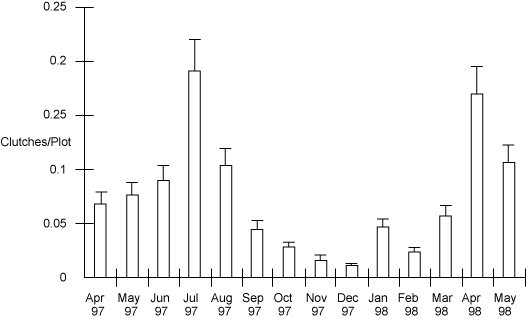
Example of a bar graph displaying biological data. Number of frog egg clutches found per plot from April 1997 to May 1998.

A line graph is constructed by connecting the data points with a line. It can be effectively used for depicting changes over time or space. This type of graph places more emphasis on trends and the relationship among data points and less emphasis on any particular data point.

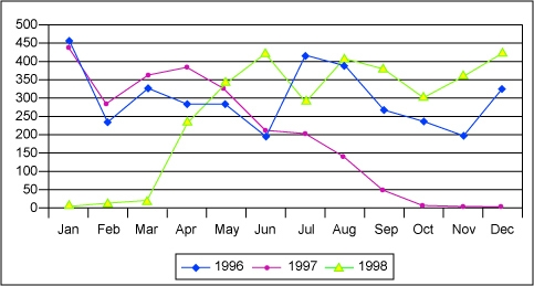
Example of a line graph used correctly to show the large impact of the 1997–98 El Niño Southern Oscillation effect on precipitation on the island of New Guinea.

Pie charts can be used to compare different categories within data relative to all categories. The proportion of each category is represented by the size of the wedge or piece of the pie. Pie charts have become popular because they are useful and simple. See the example below showing the relative proportions of clutches from different kinds of frogs found in the 1998 field season.

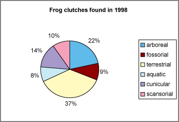
This pie chart accurately shows the different numbers of frog clutches found in 1998. Each category is a separate microhabitat where the frogs live and lay their eggs.

Graphing Tips

No matter what kind of figure you use, there are some good guidelines to follow so that you can use them most effectively. Each figure should have a clear function and should be easily interpreted. Every good figure relates directly to the content and context of the subject matter. Another important thing to keep in mind is bias. Like any other part of science, bias needs to be a major concern during the presentation of results, so that no distortions or introduced ambiguities negatively affect the presentation of your results. No matter what, we need to make sure that the accuracy of the results is portrayed correctly and clearly.

The data in a figure should be proportional to the real data; labeling should be clear and accurate; and the data themselves should be easily interpreted from the figure directly or via the figure legend. Never overcrowd the axes of a graph or the legend of a figure. If you think there might be any possibility of misinterpreting the figure, redo it. Figures are often your best tool for relaying complex information or large amounts of data. They are worth the extra time and effort you put into them and you should encourage your students to appreciate this.

Try to keep it simple. A basic rule is to use the least amount of ink or pixels per/datum. The more complex a figure, the greater the chances that people will either misinterpret your data or not understand what you are trying to show.

Limit the number of parts in a figure. For example, line graphs should have fewer than five lines, pie charts should be limited to five or six wedges, and the bars of a bar graph should not be too crowded.

Consider the size of the graph and select even, appropriate intervals on both axes that provide maximum exposure and expression of the data. You want the reader or viewer to be able to extract the necessary data with ease and efficiency. Figures that are too small or too crowded only make this harder and less efficient.

Create simple and short titles that adequately describe the information portrayed in the figure. Often the best titles reflect the effect of the independent variable upon the dependent variable, such as “The Effect of Light on Plant Growth.” Avoid acronyms or abbreviations unless you are absolutely certain that everyone will know what you mean. Use figure legends appropriately and do not try to put too much information or too little information in the legend. It should compliment the figure, not detract from its effectiveness.

Summary Statistics

Summary statistics are extremely useful for reducing large, unwieldy data to just a few descriptive values. They can often take pages of data and turn them into a few values that can be more quickly understood. Summary statistics are important to almost any study and include the mean, standard deviation, and number of data points (n).

Statistically, in a normal population, we usually assume a normal distribution of data points such that if a parameter is measured multiple times under the same conditions, the measurements are randomly distributed around an average with more clustering around the average than further away. A graph of the frequencies of each value typically is a bell-shaped curve for normally distributed data. As you remember from basic statistics, the mean and standard deviation determine the height and width of this curve.

Although both the mean and standard deviation are useful in describing most data, often in the natural sciences, real data do not fit a normal distribution. In these cases, we have other statistics to describe the data. Many data seem to be skewed in one direction while others have a more flattened bell shape. It is important to note that biological data, in particular, often does not follow a normal distribution because life is complex and many interdependent systems are usually affected by whatever perturbation or experimentation we attempt to force upon them. In many of these cases where the data is non-normally distributed, the mean and the standard deviation are not appropriate summary statistics and we need to either transform the data or come up with better descriptors for the non-normal data.

For describing non-normally distributed data, we use statistics that still convey the information but are not overly influenced by data points at the extremes of the distribution. The median, the range, and sometimes the interquartile range are used to describe both the central tendency and the spread of the data.

We know that the median is the value that is physically in the middle of the data set. The range is just the entire range of values from the data, and the interquartile range is the difference between the value at the 75 percent level and the value at the 25 percent level.

We can use another type of figure to help show non-normal data that encompasses these characteristics called a box and whisker plot. A box and whisker plot graphically displays the mean, median, variation, skew, range, and size of the data. In some cases, you do not need to show the quartile range if the range itself is sufficient to show the skew of the data. The whisker plot below shows how this works with data from the number of eggs in a clutch for different types of frogs.

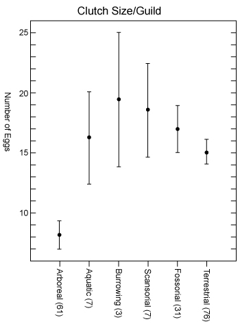
An example depicting the extreme values and median of the number of eggs per clutch across six different microhabitats. This is an example where the data are not normally distributed and need to be displayed in a slightly different way.

Maps

Displaying research results or your study area on a map is most often the best way to show where exactly the study took place or how the data are distributed geographically. A map should show the location of study sites in relation to a reference and also clearly show features, such as human habitations, rivers, major mountains, and other attributes important for the study.

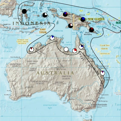
A map is best used to illustrate your results at scientific meetings or in reports when you need to show where you did your study. This map should be relatively simple and show only principal features that are cogent for the study or results. The map should have enough detail and correct scale to show location of sample sites, and whatever summary information is appropriate.

Suggestions for using a map to display your data include:

• Limit the amount of information presented.
• Clearly label the map and provide a legend to interpret it.
• Show the conclusion if you have a clear one. For example, if a map shows that gene frequencies are completely different on opposite sides of a large mountain range, use the information as a subtitle of the map and make sure that the map clearly shows the trend.
• Use an enlargement of the focal area on the map to adequately display the information and set the geography.
• Use different sized symbols and patterns to represent various magnitudes of the results. For example, a site with a sample size of 10 individuals could have a pie chart 10 mm wide whereas a sample size of 90 individuals would be 90 mm in diameter. Start by finding the highest and lowest values, assign diameters and patterns to those and then fill in steps along the way.

Exponential Relationships

Data from an experiment does not always form a line on a graph. In some changes, the amount of y increases faster and faster as the amount of x increases. In other words, it increases exponentially. A graph of exponential growth is a curve that rises increasingly faster. Exponential equations are written in the form:

N(t) = N₀e^kt

where N₀ represents the initial quantity; t represents the number of time intervals; N(t) is the quantity after time t; k is a constant that is characteristic of the growth; and e^x represents an exponential function of base e.

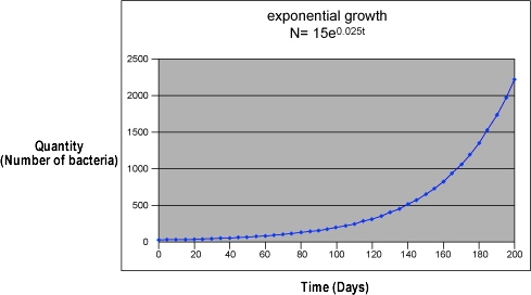
An example of exponential growth in science is uncontrolled population growth. If a bacterial culture has an unlimited food supply, its population will increase exponentially. For example, if each bacterium produces two bacteria each day, the growth will follow the pattern: 1 on the first day, 2 on the second day, 4 on the third day, 8 on the fourth day and so on. Other examples of exponential growth include the heat generated by an uncontrolled exothermic reaction, and the chain nuclear reaction of an atomic bomb.

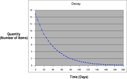
When the number of objects decreases exponentially over time, the phenomenon undergoes exponential decay. Notice that the graph of exponential decay shows an initial rapid decrease and then decreases at an increasing slower rate. Note also that the value approaches, but never crosses zero on the y-axis. An example of exponential decay is radioactive decay, in which the number of atoms of an isotope is decreased by half during a time period, known as the half-life, which is a characteristic of the particular isotope. The formula for exponential decay is:

N(t) = N₀e^-kt

Logarithmic Graphs

It is easy to read values on a graph of an exponential function when the values are changing rapidly, but when the change is slow, it is almost impossible to read the change in y on the graph with any precision. When data covers a wide range of values and rates of change, a logarithmic graph is generally more useful. The values with the wide range are plotted as the base 10 logarithm of their value.

Logarithms are used to express the magnitude of exponential functions, such as the strength of an earthquake. An earthquake of magnitude 7 is 10 times as strong as an earthquake of magnitude 6; 100 times as strong as an earthquake of magnitude 5; 1,000 times as strong as an earthquake of magnitude 4; and so on. Other values expressed logarithmically are the intensity of sound and the pH of a chemical solution.

Lab Safety

One final and very important part of doing scientific investigation is keeping yourself and others safe while you work. In many ways, safety in the laboratory is a matter of common sense. It is worthy, however, of revisiting some key elements of safety.

• Wear appropriate protective equipment, including ANSI approved safety glasses, gloves, and a lab coat whenever needed. Depending on the specific work you might be doing, there are many specific safety protocols and equipment for each situation. Make sure you know your safety issues and equipment thoroughly.
• Always review the reaction hazards and toxicity information for all chemicals you use. Consult the Material Safety Data Sheet (MSDS) for each chemical.
• Never eat or drink in the laboratory.
• Know the location of fire extinguishers, first aid kits, emergency gas and electricity shut-off valves, safety blankets, eye wash, and other safety equipment.
• Clean up spills immediately according to the MSDS procedure for that chemical.
• Maintain an uncluttered work area to prevent accidents.
• Follow approved disposal procedures for all chemicals, consult the MSDS sheets.
• Ensure that everyone you work with is also familiar with and prepared for the laboratory activity including their role in any emergency situation. A good team can save your life.
• Verify that your chemical and equipment use and storage area are compatible with the most recent Occupational and Safety Hazards (OSHA) standards.

Summary

• Science is an ongoing process that builds upon and extends our existing knowledge base.
• Mathematics is a key tool for most all scientific investigations.
• The SI metric measurement system is employed across scientific disciplines to provide consistency.
• Scientific notation and significant digits increase precision for scientific measurements.
• Precision is the exactness to which a measurement can be reproduced.
• Accuracy is the closeness of a measured value to an accepted value.
• Scientific data can be visualized through the use of tables, graphs, and maps.
• When conducting research, it is important to employ common sense and follow standard safety rules.