In this lesson we will review the experimental evidence that led to the quantum mechanical model of the atom.
By the end of the 19th century, Newtonian, or classical mechanics and classical electromagnetic theory
(summarized in what are known as Maxwell’s equations) had been used successfully to interpret matter as particulate, consisting of individual atoms, and light as an electromagnetic wave. While certain experimental observations, such as the diffraction and interference of light could be explained in terms of classical physics, the processes involved in the absorption and emission of light by matter and the interaction of positive and negative charges in the atom could not. Four unexplained phenomena were of particular importance: black body radiation, the photoelectric effect, the absorption and emission of light by atoms, and the structure and stability of the atom.
The English physicists Rayleigh and Jeans used classical electrodynamics and statistical ideas in deriving their radiation law to predict the frequency distribution expected for radiation from hot objects, called black body radiation. The Rayleigh-Jeans radiation law agreed with experiments for long wavelength, low frequency components of the distribution, but its prediction, dubbed the “ultraviolet catastrophe,” that one would observe infinite amounts of short wavelength, high frequency radiation was completely incorrect.
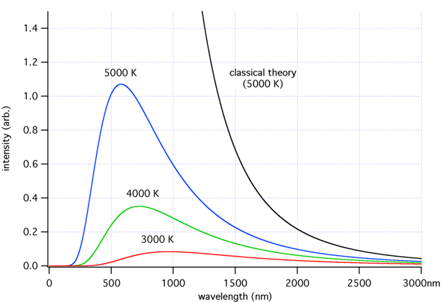
Frequency distributions for black body radiation.
The graph shows that as temperature decreases the peaks of the black body radiation curves move to lower intensities and longer wavelengths which goes against the prediction of Rayleigh and Jeans.
Quantum physics began in 1900 with Max Planck’s derivation of his radiation law, which correctly predicted the spectral distribution of a black body radiation. Planck modeled a black body as a collection of a very large number of electric charges, each of which vibrates at the same frequency ν. In contemporary terms, these charges would be electrons bound to surface atoms of the black body, and would absorb and emit electromagnetic radiation.
Planck discovered that to make his solution fit experimental results he was forced to make two assumptions. In the first of these, his quantum hypothesis, he postulated that allowed oscillator energies were multiples of a discrete amount or quantum of energy,  . Therefore an oscillator might have energy ,
  ,
,  , and so on, and could absorb or emit energy only in multiples of .
His second assumption was that ![]() is proportional to the oscillator frequency ν,
is proportional to the oscillator frequency ν, ![]() = hν. Planck chose the value of the proportionality constant h so that predictions of his model matched experimental observations. The currently accepted value of h is 6.62608 × 10⁻³⁴ J·s. Given the magnitude of Planck’s constant, the difference in energy between a quantum with energy (n)hν and one with energy (n + 1)hν is so small that the spectrum of radiation from a black body would appear to be continuous.
= hν. Planck chose the value of the proportionality constant h so that predictions of his model matched experimental observations. The currently accepted value of h is 6.62608 × 10⁻³⁴ J·s. Given the magnitude of Planck’s constant, the difference in energy between a quantum with energy (n)hν and one with energy (n + 1)hν is so small that the spectrum of radiation from a black body would appear to be continuous.
Planck’s quantum hypothesis was at complete odds with classical physics, and was not immediately accepted by Planck’s contemporaries or by Planck himself. It was only after it had successfully explained a great many phenomena that it became a part of the structure of modern physics.
When light of sufficiently short wavelength lluminates a clean surface of a metal object, the metal object becomes positively charged. This is called the photoelectric effect—electrons are ejected from the metal when short wavelength light is absorbed—and was first observed in 1887 by Wilhelm Hallwachs, a doctoral student of Heinrich Hertz, while they were studying the generation of electromagnetic waves—research which proved Maxwell’s earlier prediction that light was an electromagnetic wave.
Subsequently, Hallwachs, Philipp Lenard, who had also worked with Hertz, and the English physicist J.J. Thomson demonstrated that the effect of light on a metal was to eject electrons from the metal, but other details of the process were puzzling. The effect of ordinary waves, such as water or sound waves, depends on the amount of energy the waves deliver. This, in turn, depends on wave intensity—the amount of energy delivered per unit time per unit area—and on the time during which the wave acts, but it does not depend on the wave frequency. Increasing or decreasing either wave intensity or the interaction time increases or decreases the effect, but changing the wave frequency does not.
On the basis of classical wave theory, increasing the intensity of light should increase the kinetic energy of the ejected electrons, no matter what the frequency of the light used. However, with the photoelectric effect, light whose frequency (v) was below v0, a minimum value characteristic of the particular metal used, had no effect—no electrons were ejected, no matter what the intensity of the light. With light with a frequency (v) greater than v0, the minimum frequency necessary for electron ejection, and the kinetic energy of the ejected electrons was proportional to the difference between the frequency of the light used and the minimum frequency needed for light to eject electrons. These results could not be explained in
terms of classical mechanics.
In 1905, Einstein realized that he could explain the photoelectric effect if he extended Planck’s quantum hypothesis to light. Einstein proposed that electromagnetic energy itself is quantized, and that a beam of light consists of photons, each with energy proportional to its frequency, Ephoton = hν.
If the photon energy is less than the minimum energy needed to eject an electron, E0 = hv0, there will be no photoelectric effect.
When photons with energy equal to or greater than the minimum necessary for electron ejection (E = hν ≥ hv0 = E0) are absorbed by a metal, electrons will be ejected, and their kinetic energy (K) will be the difference between the photon energy and the minimum amount of energy required for electron ejection, K = hν – hv0.
If light of frequency 8.00 × 10¹⁴ Hz is shined on lithium, how fast will the photoelectrons that are ejected be moving?
Hints: The kinetic energy of a photoelectron is equal to the difference between the energy of the photons used, hν, and the minimum photon energy needed to eject electrons, hv0. The mass of an electron is me= 9.11 × 10⁻³¹ kg.

Solving for the speed of the electron v,
v = ![]() =
= 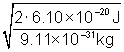 = 3.66 × 10⁵ m/s
Einstein’s explanation of the photoelectric effect meant that energy exchange between light and atoms involved quanta of energy, but there is more to the story. In 1922 A.H. Compton discovered that while photons, unlike particles, have zero mass, they are like particles in that they have momentum. In classical physics the momentum (p) of a particle is the product of its mass (m) and its velocity (v), p = mv, but a photon’s momentum is equal to Planck’s constant (h) divided by the photon wavelength (λ), p = ![]() .
.
In 1924, Louis de Broglie, a graduate student at the University of Paris, proposed that the wave-particle duality of light was true of matter as well—that if a photon has both wave and particle-like properties, a material particle should also. The de Broglie relationship between the momentum of a particle and the particle wavelength, p = ![]() , was verified in 1927 by G. P. Thomson in England and C. J. Davisson and L. Germer in the United States, who showed that beams of electrons were diffracted by thin metal films or by metal crystals in the same way as were X-rays of the same wavelength.
, was verified in 1927 by G. P. Thomson in England and C. J. Davisson and L. Germer in the United States, who showed that beams of electrons were diffracted by thin metal films or by metal crystals in the same way as were X-rays of the same wavelength.
You may find the biography of the electron amusing. J.J. Thompson demonstrated that the electron was a particle in 1897, and received the Nobel Prize for that discovery in 1906. In 1937 G. P. Thomson was awarded the Nobel Prize for his discovery in 1927 that the electron was a wave. J. J. and G.P. were father and son—so the father proved the electron was a particle and the son proved it wasn’t.
Atomic absorption and emission spectra consist of narrow lines, and so are called line or discrete spectra, as distinct from the continuous emission spectrum of light from the sun or from an incandescent lamp. Figure 2 below shows the four lines of the hydrogen emission spectrum that are in the visible region, the Balmer series of spectral lines.

Figure 2
In 1885 Johann Balmer found that the reciprocal wavelengths (![]() ) of the four hydrogen lines in the visible spectrum, all that were known then, were given by the formula:
) of the four hydrogen lines in the visible spectrum, all that were known then, were given by the formula:
![]() = R
= R![]()
where the constant R = 1.096776×10⁷ m–1 and each integral value of m >2 corresponded to a spectral line. Balmer suggested that his formula might be a special case of a more general equation, and in 1888 J. R. Rydberg and W. Ritz, working independently, found that reciprocal wavelengths for the complete hydrogen spectrum, from the infrared to the ultraviolet, are given by ![]() = R
= R![]()
where n and m are integers, with n ≥ 1, and m > n. Rydberg’s formula also applies to hydrogenic ions, ions with a single electron, such as He+, Li2+, and Be3+
Absorption and emission spectra of gaseous atoms of other elements are much more complex than the hydrogen spectrum, not surprising in light of the fact that only hydrogen has a single electron. There are no simple Rydberg-like expressions for spectral lines of elements with two or more electrons.
The amount of energy needed to remove an electron from a gaseous atom, its binding or ionization energy (IE), can be measured in a variety of ways. The first ionization energy, the energy required to remove the least tightly held electron from a gaseous atom, provides important clues about the structure of an atom.
Remember that, as we move across a row of the periodic table, the ionization energy is lowest for the first element and greatest for the last. Moving across the second and third rows of the periodic table, the ionization energy falls slightly at two points, between the second and third elements and between the fifth and sixth elements in the period. There is a gradual decrease in ionization energy as we move down a column or family of the periodic table.
The pattern of ionization energies is consistent with a simple but useful empirical model of the atom, the electron shell model, in which electrons in an atom occupy spherical shells with the nucleus at the center. Electrons in shells closer to the nucleus are held more tightly than electrons in shells farther from the nucleus.
In the electron shell model electrons in atoms of hydrogen and helium occupy the first shell, electrons in atoms of the elements lithium through neon occupy the first and second shells, electrons in atoms of sodium through argon occupy the first, second, and third shells, and with potassium and calcium we begin filling a fourth electron shell. Each electron shell is assigned a number n; n = 1 for the first shell, which is closest to the nucleus; n = 2 for the next shell, and so on.
The drops in ionization energy that occur as we move from the second to the third element and from the fifth to the sixth element in both the second and third rows of the periodic table suggest the possibility that within a given electron shell electrons can occupy subshells with somewhat different energy levels. In order to decide this question and further refine our electron shell model, we need to know how all of the electrons in an atom are distributed.
More detailed information about the arrangement and energy of individual electrons in the shells of an atom is provided by photoelectron spectroscopy (PES). This technique involves illuminating a sample of gaseous atoms with high-energy ultraviolet or X-ray photons of known energy hν. The energy of the photons used is greater than that needed to remove even the most tightly held electron from an atom, and so any electron in an atom can be ejected. Energy in excess of that needed to remove a particular electron from an atom is carried away as kinetic energy (K) by the ejected electron.
In a PES experiment two quantities are measured simultaneously; the kinetic energy K and number of ejected electrons that have that kinetic energy. The ionization energy IE is the difference between the photon energy hν and the kinetic energy K.
IE = hν – K
So the more tightly an electron is held in an atom by the attractive force of the nucleus, the larger its ionization energy and the smaller the kinetic energy of the ejected photoelectron.
The results of a PES experiment can be displayed as a spectrum of signal intensity—the magnitude of the photoelectron current—versus the ionization energy. (Note: The ionization energy decreases from left to right in a PES spectrum.) Peak heights are proportional to the number of electrons occupying a particular energy level.
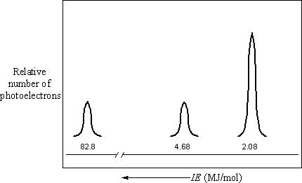
PES spectrum of neon
The figure above represents a PES spectrum of neon. There are three peaks in the spectrum of neon, at 82.8, 4.68, and 2.08 MJ/mol, with ratios of relative intensity (as compared to the intensity of the single peak in the spectrum of hydrogen) 2:2:6, respectively. The peak at 82.8 MJ/mol corresponds to two electrons occupying the n = 1 shell that is closest to the nucleus. The pattern of first ionization energies suggests that there are eight electrons in the n = 2 shell, but the PES spectrum for neon shows that these electrons occupy two subshells. The peak at 4.68 MJ/mol corresponds to two electrons in one subshell and that at 2.08 MJ/mol corresponds to six electrons in a second subshell somewhat farther from the nucleus than the first.
Table 1 summarizes experimental PES results for the first ten elements in the periodic table.
| Element/IE (MJ/mol) | 1st peak |
Relative Intensity |
2nd |
Relative Intensity |
3rd |
Relative Intensity |
|---|---|---|---|---|---|---|
|
H |
1.31 |
1 |
||||
|
He |
2.37 |
2 |
||||
|
Li |
5.28 |
2 |
0.52 |
1 |
||
|
Be |
10.7 |
2 |
0.90 |
2 |
||
|
B |
18.0 |
2 |
1.36 |
2 |
0.8 |
1 |
|
C |
27.3 |
2 |
1.72 |
2 |
1.09 |
2 |
|
N |
38.4 |
2 |
2.45 |
2 |
1.40 |
3 |
|
O |
51.1 |
2 |
2.72 |
2 |
1.31 |
4 |
|
F |
67.2 |
2 |
3.88 |
2 |
1.68 |
5 |
|
Ne |
82.8 |
2 |
4.68 |
2 |
2.08 |
6 |
| Sources: National Institute of Standards and Technology (NIST). X-ray Photoelectron Spectroscopy Database. U.S. Secretary of Commerce on behalf of the United States of America, 2003. Available online at: http://srdata.nist.gov/xps/index.htm. Spencer, Bodner and Rickard, Chemistry: Structure and Dynamics, Second Edition, John Wiley, 2003. |
||||||
Table 1: Photoelectron Ionization Energies and Peak Intensities for Gaseous Atoms of Elements 1 through 10
We have described the electron shell model for the first ten elements. Spectroscopic studies of the remaining
elements have led to an understanding of the arrangement of the electrons in atoms of every element and their
electron configurations. The structure of the electron shell model for an atom can be described using the following
rules:
Lowest energy or ground state electron configurations for the first twenty elements are as follows:
| H (Z = 1) | 1s1 | Na (Z = 11) | 1s22s22p63s1 |
| He (Z = 2) | 1s2 | Mg (Z = 12) | 1s22s22p63s2 |
| Li (Z = 3) | 1s22s1 | Al (Z = 13) | 1s22s22p63s23p1 |
| Be (Z = 4) | 1s22s2 | Si (Z = 14) | 1s22s22p63s23p2 |
| B (Z = 5) | 1s22s22p1 | P (Z = 15) | 1s22s22p63s23p3 |
| C (Z = 6) | 1s22s22p2 | S (Z = 16) | 1s22s22p63s23p4 |
| N (Z = 7) | 1s22s22p3 | Cl (Z = 17) | 1s22s22p63s23p5 |
| O (Z = 8) | 1s22s22p4 | Ar (Z = 18) | 1s22s22p63s23p6 |
| F (Z = 9) | 1s22s22p5 | K (Z = 19) | 1s22s22p63s23p64s1 |
| Ne (Z = 10) | 1s22s22p6 | Ca (Z = 20) | 1s22s22p63s23p64s2 |
Z = atomic number of the element
You can predict subshell electron populations for most of the elements with Z = 1 through 56 using the
following order of filling subshells.
There are exceptions to this order of filling among the first and second transition series elements, because the 4s and 3d subshells in the first transition series and the 5s and 4d subshells in the second transition series are very close in energy. We find that half full and completely full d subshells are more stable than other configurations. As a result, while we would predict, for example that the electron configuration for copper (Z = 29) would be 1s22s22p63s23p64s23d9, it is actually 1s22s22p63s23p64s13d10.
Interestingly, when a transition element atom ionizes, it is the electrons in the outermost s subshell that
are most easily removed. Thus, for example, the electron configuration for the Co+2 ion is 1s22s22p63s23p63d7, not 1s22s22p63s23p64s23d5.
There are two categories of electrons, core, or inner electrons, and valence, or outer shell electrons. Valence electrons in the first two elements, hydrogen and helium, occupy the first shell. The two electrons in the first shell are core electrons for the next eight elements, lithium through neon; the valence electrons of these elements occupy the second shell. In the next eight elements the ten electrons in the first and second shells are core electrons; as for the preceding eight elements, valence electrons occupy the outermost third shell. In writing electron configurations, core electrons are often represented by the symbol for the noble gas with the same electron configuration enclosed in brackets. For example, the electron configuration for silicon can be written as [Ne]3s23p2; that for potassium as [Ar]4s1.
There is a close correspondence between electron shells and the structure of the periodic table for the first 20 elements; each shell corresponds to a row of the periodic table. This correspondence between electron shells and rows of the periodic table is more complicated for transition elements, but still serves as a useful model of atomic structure.
While only valence electrons are involved in chemical bonding, there are interactions between both core electrons and the nucleus with valence electrons, and these interactions have a significant influence on the chemical properties of a given atom. As the number of core electrons increases, there is a corresponding increase in nuclear charge and in the volume core electrons occupy.
These simultaneous changes have two opposing effects on valence electrons. Because core electrons occupy shells that lie between the nucleus and the valence shell, they shield or screen valence electrons from the full charge on the nucleus. This means that the effective or core charge acting on valence electrons is smaller than the full nuclear charge. While the actual magnitude of the effective nuclear
charge that acts on valence electrons in a given atom cannot be measured, it is defined qualitatively as the sum of the positive charge on the nucleus and the negative charge of the core electrons.
Core Charge = (+Nuclear Charge) + (–Charge on Core Electrons)
Thus, for example, the core charge in an oxygen atom is +6, equal to the sum of the +8 charge on the oxygen nucleus
and the -2 charge of the two core electrons.
As the nuclear charge increases across a row, core electrons, whose numbers are fixed for elements in a given row, are pulled closer to the nucleus, reducing the volume the core electrons occupy in the atom, and allowing valence electrons to move somewhat closer to the nucleus. This and the increase in the core charge across a row means that the attractive forces acting on the valence electrons grow stronger across a row.
While attractive forces between valence electrons and the nucleus grow stronger as the charge on the nucleus increases across a row, repulsive forces between valence electrons also grow stronger as electrons are pulled closer to the nucleus and each other. However, because electrons within the valence shell do not screen each other from the charge on the nucleus as effectively as electrons in inner shells screen those in outer shells, there is a net increase in the attractive forces between the valence electrons and the nucleus in elements in a row from left to right across a row in the periodic table. As a result, on average, ionization energies increase and atomic radii decrease from left to right across a row.
As we move down a column in the periodic table, the number of filled core electron shells increases, and so the volume occupied by core electrons increase. As a result, the distance between valence electrons in the outermost shell and the nucleus increases, weakening the attraction between the nucleus and electrons in the valence shell, so ionization energies decrease and atomic radii increase from top to bottom down a column.
These trends are consistent with the decrease in metallic character of elements from left to right across a period and the increase in metallic character of elements from the top to the bottom of a group.