In this lesson we will review additional evidence leading to the quantum mechanical model of the atom.
J.J. Thomson, who discovered that the electron was a subatomic particle in 1897, proposed the “plum pudding” model of the atom (1904) in which electrons were “plums” in a “pudding” of positive charge This model was proved wrong by experiments done in 1909 by Hans Geiger and Ernest Marsden under the direction of Ernest Rutherford, who interpreted the results to mean that a large amount of the charge—positive or negative—in an atom was concentrated in a very tiny nucleus at the center of the atom. In 1911 Rutherford proposed a model of the atom in which electrons orbit a central positively charged nucleus.
Rutherford’s model of the atom had a problem. Consider the hydrogen atom. In it, the electron is acted upon by the attractive electrostatic force between it and the proton. In classical mechanics, the force acting on an object is equal to the product of mass and acceleration, F = ma; this means that the electron in a hydrogen atom must be accelerating. While this does not present a problem for analogous situations with electrically neutral objects—a planet orbiting the sun or a car accelerating down the road, for example—classical electromagnetic theory predicts that an accelerating charge must radiate electromagnetic energy. As it loses energy, the electron in a hydrogen atom should spiral into the nucleus—the atom should not be stable—and the radiation emitted should be continuous. In fact, hydrogen and all other atoms are electronically stable—their electrons do not collapse into the nucleus—and, as we have seen in Part I of this lesson, hydrogen and all other gaseous atoms both absorb and emit radiation at discrete frequencies.
Between 1913 and 1915 Niels Bohr developed a planetary model of the hydrogen atom—with the electron circling the nucleus like a planet circling the sun—that was based in part on classical mechanics and electromagnetic theory, but incorporated a quantum postulate: that the angular momentum of the electron was restricted to integral multiples of ![]() , in other words, it was quantized.
, in other words, it was quantized.
Bohr’s theory predicted that the energy of an electron in the nth energy level of a hydrogen atom is given by the expression
En = ![]() = -13.6
= -13.6
eV ![]()
where m is the electron mass, k is Coulomb’s constant (-8.37 × 10⁻¹⁹ J), e is the charge on an electron, h is Planck’s constant (6.626 × 10⁻³⁴ J·s) , and n is an integer, equal to or greater than one. Thus the energy of an electron in the lowest energy level (n = 1) is -13.6 eV, where 1 eV(an energy unit often used when dealing with atomic energy levels) is equivalent to 1.6022 × 10⁻¹⁹ J. For an electron to move from the nthallowed energy level to the mth allowed energy level of hydrogen, it would have to absorb or emit a photon whose energy was equal to the difference in energy between the two levels:
![]()
If m is greater than n, the energy change is positive and a photon is absorbed; if m is smaller than n, the energy change is negative and a photon is emitted.
Since the wavelength of light is related to its frequency (the product of wavelength and frequency is equal to the speed of light, λν = c), Bohr’s equation for the energy of a photon can be rearranged to give an expression equivalent to the Rydberg equation discussed in Part I of this lesson. Bohr found that the value he predicted for R, the constant in the Rydberg equation, was equal (within the limits of experimental uncertainties) to the experimental value for R, and the spectrum predicted by his theory was in complete agreement with experimental values for the hydrogen spectrum.
While Bohr’s theory was successful with hydrogen and hydrogen-like ions, it could not be extended to atoms with more than one electron, and it could not explain relative intensities of lines in the hydrogen spectrum. Other flaws in the theory were that Bohr’s quantum hypothesis was ad hoc—there was no fundamental basis for this assumption—and that it was based on assumptions (most significantly, electron orbits and the validity of classical mechanics and electromagnetism as applied to atoms) that could not be experimentally verified. Thus while Bohr’s theory was an important step, a completely correct theory of the atom remained to be discovered.
What is the wavelength of the photon emitted when an electron in the n = 5 energy level of hydrogen moves to the n = 2 energy level?

λ = ![]() =
= ![]() = 4.34 ×10⁻⁷ m, which is in the violet region of the visible spectrum.
= 4.34 ×10⁻⁷ m, which is in the violet region of the visible spectrum.
In 1925, Werner Heisenberg developed what came to be known as matrix mechanics, a system of atomic mechanics that uses only observable entities, such as spectral frequencies and intensities, as the basis for its calculations and which was completely successful in its applications. In spite of its successes, matrix mechanics never gained popularity, because it used mathematics that was unfamiliar to physicists and gave results that were not easily visualized.
In the fall of 1925, Erwin Schrödinger came across de Broglie’s work, and began considering a theory of the electron in an atom as a wave. Over the course of the following year, Schrödinger published a series of papers in which he presented his wave theory of atomic structure, completely different in form from Heisenberg’s matrix mechanics, but completely equivalent to it in content. While the two theories are equivalent, Schrödinger’s quantum mechanics was more palatable to physicists and became the dominant model of the electron.
While it seems quite odd that electrons, apples, and oranges should all behave like waves, we need to keep two things in mind.
First, the de Broglie wavelength is given by λ=![]() , which for an electron traveling at speeds an electron in an atom might have—say 1% of the speed of light—will be of the order of 2×10⁻¹⁰ m, or about the size of a typical atom. On the other hand, for apples and oranges traveling at ordinary apple and orange speeds the wavelength is of the order of 1 ×10-34 m or less—a wavelength that is quite unobservable!
, which for an electron traveling at speeds an electron in an atom might have—say 1% of the speed of light—will be of the order of 2×10⁻¹⁰ m, or about the size of a typical atom. On the other hand, for apples and oranges traveling at ordinary apple and orange speeds the wavelength is of the order of 1 ×10-34 m or less—a wavelength that is quite unobservable!
Second, a line spectrum of energy absorption is a characteristic of a wave that is confined in a bounded region, for example, a wave on a string stretched between two fixed points. At certain frequencies, called resonant frequencies, the string efficiently absorbs energy and a stationary or standing wave—a wave for which the locations of nodes, points at which the wave amplitude is zero, and antinodes, points at which the wave amplitude is greatest, are fixed—is established. At non-resonant frequencies, very little energy is absorbed and wave amplitude is negligible. The line absorption and emission spectra of atoms suggest that a standing wave phenomenon is involved, and since it is electrons in an atom that are involved in absorption or emission of energy, the electron as wave seems plausible.
The details of quantum mechanical calculations need not concern us here, but the basic principles, concepts, and results of quantum mechanics are fundamental to the contemporary chemist’s understanding of molecular structure, chemical properties, and chemical reactivity. Today, quantum mechanics serves as a predictive tool in the design of new materials and drugs, and a wide variety of computational software makes quantum mechanical calculations and molecular modeling accessible to anyone with a personal computer.
Schrödinger’s quantum mechanics gave results identical to the experimental results on which the electron shell model was based. He showed that electrons with different energies occupy different regions about the nucleus called orbitals.
Each orbital in an atom has a unique set of three quantum numbers, n, l, and m, that characterize, respectively, the distance of the orbital from the nucleus, the shape of the orbital, and its orientation in space. The three quantum numbers are related to each other and to the electron shell model in the following ways:
The value of l determines the type of orbital:
| l | 0 | 1 | 2 | 3 |
| Orbital | s | p | d | f |
There are orbitals corresponding to higher values of l, but we will consider only s, p, d, and f orbitals, as only these are involved in ground state electron configurations.
Each subshell has a specific value for l and within a subshell there is one orbital for each allowed value of m. For example, in a subshell with l = 0 and m = 0, there is 1 single s orbital; in a subshell with l = 1 and m = 1, 0, or -1, there are three p orbitals. Orbitals are labeled with their principal quantum number and orbital type; for example the label for an orbital with
n = 2 and l = 1 is 2p. Table 1 lists the allowed combinations of quantum numbers for n = 1, 2, 3, and 4, the orbital type and number of orbitals in a subshell, and the number of electrons in a full subshell.
| Shell (n) |
Subshell (l)
|
Orbital (m)
|
Orbital Notation
|
Number of Orbitals in Subshell
|
Number of Electrons in Full Subshell
|
|---|---|---|---|---|---|
|
1
|
0
|
0
|
1s
|
1
|
2
|
|
2
|
0
|
0
|
2s
|
1
|
2
|
|
2
|
1
|
1, 0, -1
|
2p
|
3
|
6
|
|
3
|
0
|
0
|
3s
|
1
|
2
|
|
3
|
1
|
1, 0, -1
|
3p
|
3
|
6
|
|
3
|
2
|
2, 1, 0, -1, -2
|
3d
|
5
|
10
|
|
4
|
0
|
0
|
4s
|
1
|
2
|
|
4
|
1
|
1, 0, -1
|
4p
|
3
|
6
|
|
4
|
2
|
2, 1, 0, -1, -2
|
4d
|
5
|
10
|
|
4
|
3
|
3, 2, 1, 0, -1, -2, -3
|
4f
|
7
|
14
|
Table 1
Below are sketches of s, p, and d orbitals. Each value of m corresponds to a unique orbital orientation. For example, for l = 1, there are three p orbitals, one for each allowed value of m, 1, 0, and -1. These are usually labeled as px, py, and pz, where the subscripts specify the shapes and orientations of the orbitals. Thus, for example, an electron in a pz orbital is confined to a region above and below the x-y plane and centered around the z-axis. The shapes and orientations of d orbitals
are more complex. For example, a dxy orbital has four lobes that lie in the x-y plane between the x and y axes, and a ![]() orbital has four lobes that lie along the x- and y-axes.
orbital has four lobes that lie along the x- and y-axes.
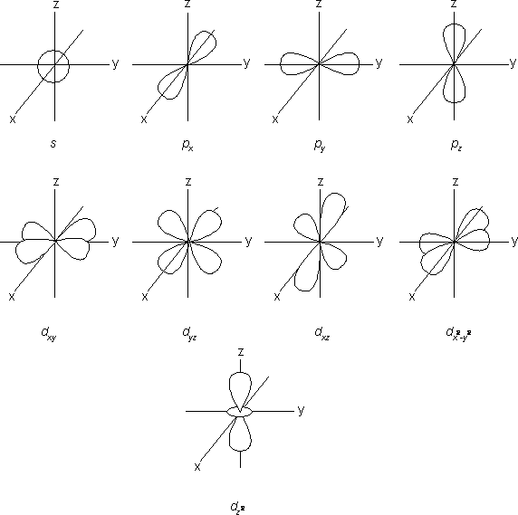
Sketches of s, p, and d orbitals
Without consulting Table 1, answer the following questions:
a) If n = 4, l can have values 3, 2, 1, or 0, so there will be one 4s orbital, three 4p orbitals, five 4d orbitals, and seven 4f orbitals, for a total of sixteen orbitals.
b) The l =3 subshell is composed of seven f orbitals.
c) The l = 3 subshell can hold fourteen electrons.
At this point, the empirical electron shell model we developed in Part I of this lesson is essentially equivalent to the electron shell model based on quantum mechanics. Though we now know that p, d, and f subshells have multiple orbitals, we do not know how electrons in one of these subshells are distributed among these orbitals. The key to understanding how electrons are arranged in the orbitals of a subshell involves a fourth, two-valued quantum number s, introduced by Wolfgang Pauli in 1924 to explain the splitting of lines in atomic spectra into closely-spaced pairs. The physical significance of this fourth quantum number was unknown at this point.
Otto Stern and Walter Gerlach had discovered in 1922 that a beam of silver atoms was split into two parts by an inhomogeneous magnetic field, an effect that indicated that silver atoms acted like atomic magnets. The fact that the beam was split into two parts rather than simply broadened, suggested that two quantum magnetic states were involved.
In 1925, Ralph Kronig, a graduate student at Columbia University, and George Uhlenbeck and Samuel Goudsmit, graduate students at the University of Leiden, independently explained the Stern-Gerlach results by suggested that electrons
act like rotating spheres of electric charge which behave like magnets and which, in an inhomogeneous magnetic field, will be in one of two energy levels. In an atom with an even number of electrons, these tiny magnets would form pairs that would not be affected by passing through a magnetic field. In atoms like silver, which have an odd number of electrons, there would be one unpaired electron, and a magnetic field would separate a beam of atoms into two parts.
Later in 1925, Pauli showed that his fourth quantum number s identified the spin state of the electron, electron spin up with s = +½ or electron spin down with s = -½, and developed his exclusion principle to explain a variety of experimental results. The exclusion principle specifies that each electron in an atom must have a unique set of four quantum numbers. If two electrons occupy a single orbital, each has the same values of n, l, and m, so one electron must have s=+½ and the other s
=–½ , (i.e. with spins “paired”) which means that no more than two electrons can occupy the same orbital.
With the exclusion principle and the assumption that as electrons are added to an atom they fill the lowest energy orbitals first (the “building up” or aufbau rule), we can predict the order in which electrons will go into orbitals. For example, the first and second electrons added to a carbon atom will go into the 1s orbital, filling it. The third and fourth electrons fill the 2s orbital, and the next two electrons have a choice of 2px, 2py, and 2pz, orbitals to occupy.
However, while the exclusion principle specifies that no more than two electrons can be in the same orbital, it does not tell us which arrangement of valence electrons is most stable. Thus, we cannot decide on the basis of the exclusion principle or the aufbau rule whether a carbon atom with two 2p electrons will have both in the same 2p orbital with paired spins, or in separate 2p orbitals with paired spins, or in separate orbitals with unpaired spins. To answer this question, we must apply a rule devised by Friedrich Hund, also in 1925.
Hund’s rule says (1) that there must one electron in each orbital of a subshell before any electrons are paired in any orbital of that subshell, and (2) that all electrons in a subshell have the same spin until each orbital in the subshell has at least one electron. For example, in the second shell of carbon, the 2s orbital has two paired electrons, but the two 2p electrons occupy separate 2p orbitals and are unpaired.
The usual explanation of Hund’s rule is that by occupying separate orbitals in a subshell electron-electron repulsion is minimized, and this lowers the energy of these electrons. In general, this is not correct, as very accurate calculations show that in most cases the average distance between unpaired electrons in separate orbitals is actually slightly less than that between paired electrons in a single orbital. This means that electron-electron repulsion is actually slightly greater between unpaired electrons in different orbitals than between paired electrons in a single orbital.
What does account for the stability of unpaired electrons is that screening of the nuclear charge by electrons in a subshell is reduced when they occupy separate orbitals, so the attractive forces between electrons and the nucleus are greater when electrons are in different orbitals. It is this increase in the nuclear attraction that allows unpaired electrons occupying separate orbitals in a subshell to be closer to the nucleus, making them more stable.
With our rules for placing electrons in atoms we can now predict electron configurations that include the number of electrons in orbitals. We can use the order-of-filling sequence we presented in Part I of this lesson.
If a periodic table is handy you need not memorize this scheme for filling subshells, because it can be deduced from the structure of the periodic table. For example, moving across the first row of the periodic table the 1s subshell is filled; moving across the second and third rows the 2s and 2p and 3s and 3p subshells, respectively, are filled. With the fourth row, the 4s subshell is filled, then the 3d subshell, and lastly the 4p subshell. This is the same order of filling outlined in the scheme above.
A few examples should serve to make clear what is involved:
The Ground State Electron Configuration in Oxygen
The ground state electron configuration of an oxygen atom can be written [He]2s22px22py12pz1. The assignment here of two electrons to a 2px orbital and one each to 2py and 2pz orbitals is arbitrary; what is important is that one 2p orbital is full and two are half full.
Ground State Electron Configurations in Vanadium and Chromium
The electron configuration of vanadium can be written [Ar]4s23dxy13dyz13dxz1. As with oxygen, the choice of orbitals is arbitrary; the significant point is that there are three 3d orbitals that are singly occupied. More commonly, the electron configuration in vanadium is written [Ar]3d34s2, which reflects the fact that the 4s electrons are least tightly held and lie above the 3d electrons energetically.
The next element in the periodic table is chromium, for which we might expect a ground state electron configuration [Ar]3d44s2. Spectroscopic results show that the ground state electron configuration is actually [Ar]3d54s1, with a half filled set of d orbitals.
Variation in the electron configurations for the transition metal elements in rows 5-7 of the periodic table is greater, and no simple pattern can be used to predict actual electron arrangements.
Predict the electron configurations for the following ions:
a) The electron configuration for Cu+1 is [Ar]3d10. Copper, [Ar]3d104s1, loses its single 4s electron to form the Cu+1 ion.
b) The electron configuration for Cu+2 is [Ar]3d9. Copper loses its 4s electron and one 3d electron to form the Cu+2 ion.
c) The electron configuration for Fe+2 is [Ar]3d6. Iron, [Ar]3d64s2, loses both 4s electrons to form the Fe+2 ion.
We conclude our lesson on quantum mechanics with a brief discussion of one last concept, Heisenberg’s uncertainty principle. In classical physics it is, in theory, possible to determine precisely the initial state of a system, and from this information predict the behavior of the system as far into the future as desired. However, there is a fundamental limit to the precision with which we can determine the location or momentum of any particle. Heisenberg made a careful analysis of the relationship between the uncertainty in the momentum of a particle, Δp, and the uncertainty in its location, Δx, and concluded that the product of the two was of the order of Planck’s constant h:
Δp·Δx ≈ h
The fact that atoms do not collapse can be considered a consequence of the uncertainty principle. Forcing the electrons closer to the nucleus means that Δx is reduced, which causes a larger uncertainty Δp in the momentum. While a proof is beyond the scope of this lesson, it can be shown that applying the uncertainty principle leads to a correct prediction of the dimensions of an atom.