Limits and Continuity

Objective

In this lesson, you will study limits of functions and the continuity of functions as a prerequisite to understanding differential calculus.

What is the limit of a function?

The limit of a function is the value of the function as its variable approaches a number. The expression is read the limit of as x approaches a is B. Note that must be defined everywhere along an open interval around a (which does not necessarily include a).

An example of a formal definition for a limit is:
For every number in an open interval around a (except perhaps a itself), the limit exists if, for any , there exists such that .

In other words, approaches the limit B as x approaches a, if the absolute value of the difference between and B can be made smaller and smaller as x approaches a.

There is a subtle, but very important detail within this definition. When we refer to an open interval around a, it is important to note that an open interval around a point a contains, by definition, points on either side of a. Because we only have one limit B for each a in the domain of our function, B must have the same value whether we approach a from the left or right side.

The simplest method to compute the limit of a function, whenever possible, is to plug in the value of a and see if the limit describes a real value. For example, what is ? Note that the function is not defined at since that would lead to division by zero. However, we are interested in the open interval around , so simply substituting this value of x will work.

Just because this function is not defined at , does not mean that this limit does not exist as . The limit still exists. This can be proven in several ways. One method is to substitute values close to and on either side of –3 and see what results. This method is not a formal proof, but it is convincing enough for simple functions like these. Using a calculator, compute the value of the limit at and . The results are –1.001 and –0.999, respectively. As you try values even closer to –3, your will see that your answers get even closer to –1.

A second method is to graph the function.

A third method is to simplify the function, when possible. Note that can be factored as . Therefore, the limit can be rewritten

Remember from algebra that you can cancel out similar terms in the numerator and denominator, as long as the value of the denominator is never zero. As you can see, the denominator is zero at . We are looking at values as approaches – 3, but never at . Therefore, it is safe to cancel these terms.

Unlike the plug-in method described above, this method serves as proof that the limit is indeed – 1.

Now, let’s consider . At , we see that . Does this mean that ?
According to our definition of a limit, the answer is no. The function does not have to be defined at for the limit to exist. It must exist in an open interval around . While that is true for (that is, to the right of zero), we know that the function
is not defined for (to the left of zero), since the result is the square root of a negative number.

A one-sided limit exists if is restricted in one direction but not the other. For this example, if x is restricted on the right, we say that we have a right-hand limit or a one-sided limit from the right. This is written . A left-hand limit or a one-sided limit from the left is written .

Question

Consider the piecewise function . Which statement is true for this function?

1. 

2. is not defined
3. 
4. 

Reveal Answer

The correct choice is B. Although at , the value of the function changes in the open interval to the left and right of 0. Therefore, B is true. Choices C and D are reversed; they would be correct if the signs of their limits were swapped, or if the signs above their zeroes were swapped.

Let’s look at the functions and . Below are their graphs:

f(x)		g(x)

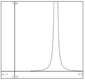
We see from the graph of that, as approaches 3 from either the right or left, blows up, or approaches infinity. This is written

and .

In this case, we say that increases without bound. Since this is true for the open interval around 3 (but not including ), we can write . This is an example of an infinite limit. This does not mean the limit exists but gives us a more descriptive way of explaining why the limit doesn’t exist. Note that if we substitute , this limit approaches as approaches 3. In this case, we say that the limit decreases without bound.

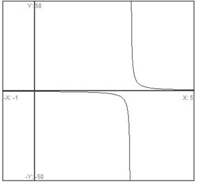
One-sided limits can also be infinite limits, as seen by . From the graph, it is clear that and . The limit decreases without bound to the left of , and increases without bound to the right of .

Not to be confused with an infinite limit, there is also a limit at infinity. The limit as approaches infinity (or negative infinity) exists if the value of approaches B as increases (or decreases) without bound. Limits at infinity are written .

Consider the function . Below is a graph of this function.

(a) Is there an infinite limit to this function for some value of x?

(b) Is the limit at x = 4 one-sided or two-sided?

(c) What are the limits at infinity (positive and negative)?

(a) Yes, as x approaches 4 from the left and right, the function blows up negatively and positively, respectively.

(b) Since the limits to the left and right of are different, the two-sided limit does not exist. We can write the one-sided infinite limits as and .

(c) . The asymptote at y = 5 is an indication of this limit at infinity. To better understand this answer, note that, as becomes very large, the denominator looks more and more like . (For example, if Bill Gates has $40 billion and loses $4 playing poker, he still essentially has $40 billion.) Therefore, as :

As , the same condition holds.

What are the limit theorems?

The following theorems involve the limits of sums, products, quotients, and compositions of functions. While they are very useful, keep in mind that these theorems are only true when the individual limits and both exist. These theorems will come in handy as we prove some important rules in differential calculus.

These theorems can be proved using the formal definition of a limit (the one with the Greek symbols). As an example, let’s prove theorem 2.

Assume and . To prove this theorem, we need to show that, for any , there exists a such that whenever .

Since , we know that, for , there exists such that whenever .

Likewise, since , we know that, for , there exists such that whenever . Since can be arbitrarily small, we can replace both with , which is the smaller of the two.

Therefore, whenever .

What are the special trigonometric limits?

There are three special limits that are important in dealing with trigonometric functions. They can be derived using trigonometry, as well as a rule that specifically deals with functions that reduce to or , which will be discussed later. For now, simply memorize the three rules.

In order to understand the basis of differential calculus, it is important to understand both limits and the continuity of a function. A function is continuous in a range where there are no breaks in the graph. If you can draw its graph without lifting your pencil, the function is continuous in this region.

Now let’s put the concept of continuity into mathematical form. A function is continuous at the value x = a if and only if the following three rules hold:

If any of these 3 conditions fail, the function is discontinuous at that value.

Continuity is a relatively simple concept. Just remember that the root word of continuous and continuity is continue. If the graph does not continue at all points, it is not continuous. Also, keep in mind that no function is continuous at a point where its denominator is zero. Thus, the function we previously examined, , is not continuous at all values, even though we showed that this function reduces to when . This function violates rule 2 at , and is discontinuous at this point.

If two functions and are continuous at , then their sum, difference, product, and quotient are all continuous at (for the quotient, ).

We may need to describe the interval over which a function is continuous. There are three terms that can describe these intervals. A function is continuous over an open interval (a, b) if the above 3 rules apply to all values between a and b, but not necessarily including a and b themselves. If the function is continuous at a and b, we say it is continuous over the closed interval [a, b]. Some functions are half-open, meaning they include one extreme but not the other— but not , for example. In this case, we say the function is continuous on [a, b).

Question

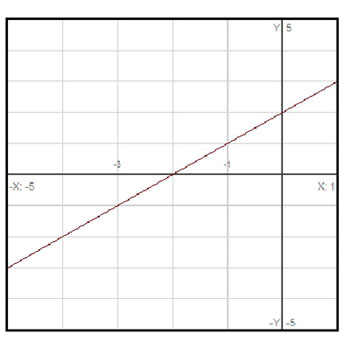
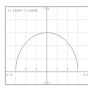
Over what interval is the function continuous?

The graph is depicted below.

Reveal Answer

This function is continuous for all where is defined. Since the square root of a negative number has no real value, we know the function is continuous at all points between and . Is the interval closed, open, or half-open? The interval is closed. at and , so we can say that is continuous on the interval .

For some discontinuous functions, the conditions can be altered to make them continuous. This results in a removable discontinuity. For example, consider the function . We know that the function is discontinuous at . We also know that . Suppose we define a new function , such that:

The function is continuous for all values of x.

Now that we understand continuity in a closed interval, we can discuss the Intermediate Value Theorem.

This theorem can be used to verify that there is a root (or zero value) for a polynomial function in a particular interval. For example, we may not be able to easily solve for the roots of . However, since we know is continuous, , and , we know by the Intermediate Value Theorem that there is at least one value for in the range where (the actual value is between and ).

As long as the function is continuous (no pencil-lifting), there will be some intermediate value between the extreme points of the function where the function is defined for a particular value of .

Another theorem, the Extreme Value Theorem is useful in understanding maximum and minimum values of a function. Given an interval for , the absolute maximum is the value for which the function is at its greatest. Likewise, the absolute minimum is the smallest value for the function in the given interval. In math-speak, has an absolute maximum in an interval if for all values of in the interval. Flip the sign, and you have the definition of the absolute minimum.

Given that definition, the Extreme Value Theorem states that, if a function is continuous on the closed interval [a, b], then has both an absolute maximum and absolute minimum in .