In this lesson, you will cover the definition of a derivative and apply it to the evaluation of slopes and tangent lines of curves, instantaneous rates of changes of functions, relative maxima and minima, and methods to compute the derivative of several types of functions.
A derivative is nothing more than a special type of limit. However, it has many important applications and interpretations. Substitute ![]() for
for ![]() in our limit equation. We usually denote the derivative of
in our limit equation. We usually denote the derivative of ![]() as
as ![]() and define it as:
and define it as:
![]() .
.
Given ![]() , where
, where ![]() are constants, compute
are constants, compute ![]() .
.
We will use the above limit to compute the derivative. First, we need to compute ![]() .
.
![]()
Therefore, ![]() . Hence,
. Hence, ![]() . Finally, we simply plug in values to find the derivative.
. Finally, we simply plug in values to find the derivative.
![]() . We will use this derivation for a couple of examples, so keep this solution handy.
. We will use this derivation for a couple of examples, so keep this solution handy.
Let ![]() , where
, where ![]() is a constant for all values of
is a constant for all values of ![]() . That means
. That means ![]() as well. Therefore,
as well. Therefore, ![]() . So the derivative of a constant is zero.
. So the derivative of a constant is zero.
Compute ![]() for
for
(A) ![]() ; and
; and
(B) ![]() .
.
Hint: Remember the two limits for ![]() and
and ![]() for small values of
for small values of ![]() . Also, recall the following trigonometric identities:
. Also, recall the following trigonometric identities:
![]()
(A) ![]()
(B) ![]()
These two derivatives are significant to many applications in calculus and should be memorized.
The derivative of ![]() is
is ![]() .
.
The derivative of ![]() is
is ![]() .
.
If a function is in the form ![]() , recall that the graph crosses the y-axis at the y-intercept
, recall that the graph crosses the y-axis at the y-intercept ![]() and has a constant slope
and has a constant slope ![]() .
.
The concept of slope is not limited to straight lines. Curves can have slopes as well, but the value of the slope of the curve ![]() changes as
changes as ![]() varies. As you may have guessed by now, the slope of the curve
varies. As you may have guessed by now, the slope of the curve ![]() at any point
at any point ![]() is defined by
is defined by ![]() . (Actually, the slope is not always defined; at these points, the value of
. (Actually, the slope is not always defined; at these points, the value of ![]() is not defined.) Below we will show why.
is not defined.) Below we will show why.
Consider the curve below and the line intersecting the curve at points ![]() and
and ![]() .
.
A line that intersects the curve at two points is known as a secant line. The slope of that line is given by:
![]()
Here, we define ![]() . Therefore, we can rewrite the above equation as:
. Therefore, we can rewrite the above equation as:
![]()
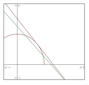
Let’s re-examine the above graph with another line that intersects the curve at just one point. This new line is known as the tangent line at the point of intersection, and describes the slope of the curve at that point. As you can see, it does not have the same slope as the secant line.
Imagine shifting the secant line so that the points of intersection become closer and closer to the tangent point. The slope of the secant line is still described by the above equation, but the value of ![]() gets smaller and smaller. In fact, the slope of the secant line and tangent line become identical as
gets smaller and smaller. In fact, the slope of the secant line and tangent line become identical as ![]() . We cannot simply plug in
. We cannot simply plug in ![]() , because it would result in a zero in the denominator. What we can do, however, is consider the limitof the value of
, because it would result in a zero in the denominator. What we can do, however, is consider the limitof the value of ![]() as
as ![]() approaches zero.
approaches zero.
![]() , which is precisely the value of
, which is precisely the value of ![]() .
.
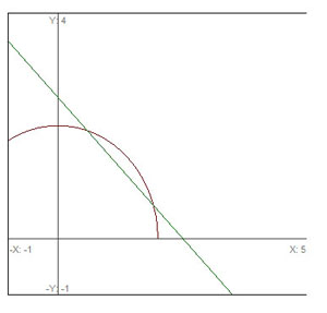
For example, given ![]() , what is the slope of the curve at
, what is the slope of the curve at ![]() ?
?
The graph of ![]() and its tangent line at
and its tangent line at ![]() are depicted below.
are depicted below.
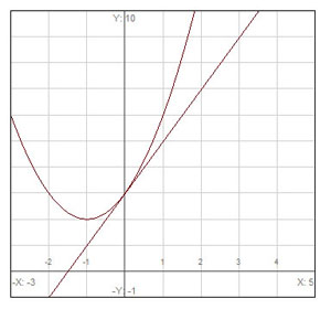
It appears that the tangent line intersects the x-axis at ![]() and the y-axis at
and the y-axis at ![]() . From these points, it appears that the slope is
. From these points, it appears that the slope is ![]() . We can verify this by taking the derivative of
. We can verify this by taking the derivative of ![]() and plugging in
and plugging in ![]() . We already calculated the derivative:
. We already calculated the derivative: ![]() . At
. At ![]() ,
, ![]() .
.
Now that we understand that the derivative of a function is equivalent to the slope of a function at a point (or to the entire function, if the function describes a line), it should be easy to equate it to a rate of change. Recall that the slope of a line is defined as ![]() . In this form, the slope describes the rate of change in
. In this form, the slope describes the rate of change in ![]() with respect to
with respect to ![]() . In physics applications, we associate the words rate of change with time. In economics, rate of change might be associated with the rate of change of cost (such as marginal cost).
. In physics applications, we associate the words rate of change with time. In economics, rate of change might be associated with the rate of change of cost (such as marginal cost).
Let’s start with a physics example. Suppose the position of a particle over time can be described by the equation ![]() , where
, where ![]() is measured in meters and
is measured in meters and ![]() in seconds. At time
in seconds. At time ![]() , the particle is at a position
, the particle is at a position ![]() (think of a race car starting
(think of a race car starting ![]() meters behind the starting line). Also note that, as
meters behind the starting line). Also note that, as ![]() increases, the value of
increases, the value of ![]() not only grows, but grows at a greater and greater rate (we usually do not look at
not only grows, but grows at a greater and greater rate (we usually do not look at ![]() .
.
For example, what is theaverage velocity of the particle from ![]() to
to ![]() seconds? Recall from algebra that rate (velocity) = distance/time. Between
seconds? Recall from algebra that rate (velocity) = distance/time. Between ![]() and
and ![]() seconds, the particle has moved from position
seconds, the particle has moved from position ![]() meters to
meters to ![]() meters, for a total of
meters, for a total of ![]() m. This distance is covered over a period of
m. This distance is covered over a period of ![]() seconds. Therefore, the average velocity is 26/2 = 13 meters per second.
seconds. Therefore, the average velocity is 26/2 = 13 meters per second.
We see that the average velocity over a time ![]() is described by:
is described by:
![]() .
. ![]() and
and ![]() sec. What happens as
sec. What happens as ![]() gets smaller and smaller? We can then measure the small change in position over a small interval in time. The average velocity then becomes close to the instantaneous velocity around that time. The instantaneous velocity is
gets smaller and smaller? We can then measure the small change in position over a small interval in time. The average velocity then becomes close to the instantaneous velocity around that time. The instantaneous velocity is ![]() as
as ![]() approaches zero, or:
approaches zero, or:
![]() . Note that this is the formula for a derivative. Except we now use
. Note that this is the formula for a derivative. Except we now use ![]() instead of
instead of ![]() , and the variable is
, and the variable is ![]() instead of
instead of ![]() . We can therefore denote
. We can therefore denote ![]() by the terms
by the terms ![]() or
or ![]() . Rather than expand the limit term, let’s just borrow what we found in the first example. For the function
. Rather than expand the limit term, let’s just borrow what we found in the first example. For the function ![]() , we found
, we found ![]() . Just substitute
. Just substitute ![]() ,
, ![]() , and
, and ![]() (as well as changing
(as well as changing ![]() to
to ![]() and
and ![]() to
to ![]() ). We find:
). We find: ![]() . This equation describes the instantaneous velocity at all times. At
. This equation describes the instantaneous velocity at all times. At ![]() second,
second, ![]() meters per second.
meters per second.
The acceleration is defined as the change in velocity over time. Using similar reasoning to find the instantaneous velocity, the acceleration ![]() is computed by taking the time derivative of the velocity:
is computed by taking the time derivative of the velocity:
![]()
Since ![]() , we can substitute
, we can substitute ![]() ,
, ![]() , and
, and ![]() into the example formula to find
into the example formula to find ![]() . If you are familiar with physics, you may recognize
. If you are familiar with physics, you may recognize ![]() as an approximation for the acceleration due to gravity.
as an approximation for the acceleration due to gravity.
A function ![]() is continuous at the value
is continuous at the value ![]() if and only if the following three rules hold.
if and only if the following three rules hold.
A function is discontinuous along an interval if there are any breaks in the graph. If the value of the function shifts at a point, if the function is not defined at a point, or if the function increases or decreases without bound at a point (as indicated by a vertical asymptote) the function is discontinuous.
The slope (i.e. the derivative) of a curve is not always defined at all points on a continuous curve. A classic example of this is the absolute value function. Below is a graph of ![]() .
.
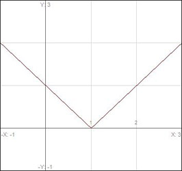
What is the value of ![]() at
at ![]() ? It is clear that the function is defined at
? It is clear that the function is defined at ![]() . The derivative is a limit, and this limit must be defined in an open interval around the point
. The derivative is a limit, and this limit must be defined in an open interval around the point ![]() . However, no matter how small we make the open interval around
. However, no matter how small we make the open interval around ![]() , the slope of the curve in the portion of the open interval to the left of
, the slope of the curve in the portion of the open interval to the left of ![]() will always be a negative number, and the slope of the curve in the portion of the open interval to the right of
will always be a negative number, and the slope of the curve in the portion of the open interval to the right of ![]() will always be a positive number, so the limit is not defined since the limit from the right hand and left hand sides do not agree. You can also see this graphically. The tangent line must intersect the curve only at one point:
will always be a positive number, so the limit is not defined since the limit from the right hand and left hand sides do not agree. You can also see this graphically. The tangent line must intersect the curve only at one point: ![]() . Prove to yourself that there are an infinite number of lines, all with different slopes, which could be described as a tangent line (any line that touches
. Prove to yourself that there are an infinite number of lines, all with different slopes, which could be described as a tangent line (any line that touches ![]() but does not penetrate the ‘V’). Be wary whenever you see a sharp turn or “pointy” graph when evaluating derivatives because the derivative will not exist at these sharp points or “cusps”.
but does not penetrate the ‘V’). Be wary whenever you see a sharp turn or “pointy” graph when evaluating derivatives because the derivative will not exist at these sharp points or “cusps”.
Another example of an undefined derivative is at a point of discontinuity. If a function is discontinuous at a point, there is no derivative at that point.
Some functions are not differentiable at a certain point because the derivative increases or decreases without bound. One example is ![]() . Below is the graph of
. Below is the graph of ![]() around
around ![]() .
.

At ![]() , the slope becomes infinite or vertical, so
, the slope becomes infinite or vertical, so ![]() is not defined there. In fact, we will later prove that any function
is not defined there. In fact, we will later prove that any function ![]() , where
, where ![]() , will have an undefined derivative at
, will have an undefined derivative at ![]() .
.
We see that a function can be continuous at all points, while ![]() can be discontinuous at a point. This is , evidenced by “pointy” functions such as
can be discontinuous at a point. This is , evidenced by “pointy” functions such as ![]() and functions whose derivatives have a vertical tangent line at a point such as
and functions whose derivatives have a vertical tangent line at a point such as ![]() . However, if a function
. However, if a function ![]() is differentiable at
is differentiable at ![]() , then it is also continuous at
, then it is also continuous at ![]() . In other words, differentiability always implies continuity, but continuity does not always imply differentiability.
. In other words, differentiability always implies continuity, but continuity does not always imply differentiability.
If two functions ![]() and
and ![]() are differentiable, the following rules apply.
are differentiable, the following rules apply.
These rules are proven below.
Proof for rule 1:
Proof for rule 2:
We can prove rule 3, or the quotient rule, using the limit definition of derivatives as well. However, the quotient rule can be derived from the product rule (rule 2), by changing ![]() to
to ![]() . Once we learn the general rule for differentiation of powers and an important rule for the derivative of composite functions known as the chain rule, the quotient rule can be easily derived from the product rule. Hence, it may not be necessary to memorize the quotient rule.
. Once we learn the general rule for differentiation of powers and an important rule for the derivative of composite functions known as the chain rule, the quotient rule can be easily derived from the product rule. Hence, it may not be necessary to memorize the quotient rule.
Before we proceed with examples, let’s learn three more important rules for derivatives:
Proof for rule 4:
Proof for rule 5:
We can factor (x + Δx)n by using the Binomial Theorem.
![]()
Look carefully at the numerator. You can see that the term in parentheses breaks down into an xn-term (which cancels out) and a series of terms with ![]() etc. Since we divide the numerator by
etc. Since we divide the numerator by ![]() , the only term we are interested in is the
, the only term we are interested in is the ![]() -term. All the others will have
-term. All the others will have ![]() to some power
to some power ![]() . Since the limit is for
. Since the limit is for ![]() , all these will zero out. What we are left with is the coefficient in front of
, all these will zero out. What we are left with is the coefficient in front of ![]() . According to the Binomial Theorem, that term is
. According to the Binomial Theorem, that term is ![]() . Therefore,
. Therefore, ![]() .
.
Proof for rule 6:
Applying the quotient rule and the power rule (rule 5) we just derived, we find that
![]()
Let’s try an example. Given ![]() , compute
, compute ![]() .
.
We will apply several of the above rules to solve this derivative. First, rule 1 tells us that we can treat each of the 4 terms separately. We won’t need to separate terms like this in the future, but for now:
Therefore, ![]() .
.
The first term can be solved by combining rules 4 and 5.
![]()
The second term uses one of the memorized trigonometric derivatives.
![]() .
.
The third term combines rules 4 and 6.
![]()
The fourth term is easier to solve with the ![]() -term separated from the variable.
-term separated from the variable.
![]() .
.
Therefore, ![]()
![]()
![]() .
.
Let’s try another example. Given ![]() , compute
, compute ![]() .
.
One method to compute ![]() is to factor the terms and derive a single polynomial expression. However, we can also use the product rule. Let
is to factor the terms and derive a single polynomial expression. However, we can also use the product rule. Let ![]() , and
, and ![]() . Terefore,
. Terefore, ![]() , and
, and ![]() .
.
Try one final example. Let ![]() . If at least one of the terms can be expressed as
. If at least one of the terms can be expressed as ![]() , where
, where ![]() is a constant and
is a constant and ![]() , show that
, show that ![]() is not differentiable at
is not differentiable at ![]() .
.
The derivative of ![]() is the sum of the derivatives of the terms, including
is the sum of the derivatives of the terms, including ![]() . From rules
. From rules ![]() and
and ![]() ,
, ![]() , where
, where ![]() is a constant. Since
is a constant. Since ![]() ,
, ![]() . That means the exponent in the derivative expression is negative. Therefore, we can rewrite the derivative as
. That means the exponent in the derivative expression is negative. Therefore, we can rewrite the derivative as ![]() , where
, where ![]() is a positive number. At
is a positive number. At ![]() ,
, ![]() does not exist, since we have division by zero. Since at least one term in the function is not differentiable, the whole expression is not differentiable.
does not exist, since we have division by zero. Since at least one term in the function is not differentiable, the whole expression is not differentiable.
A composite function is a function of a function. Given two functions ![]() and
and ![]() , the composite function is often denoted as
, the composite function is often denoted as ![]() or
or ![]() . For example, the function
. For example, the function ![]() can be considered a composite function
can be considered a composite function ![]() , where
, where ![]() , and
, and ![]() . Alternatively, we can have
. Alternatively, we can have ![]() and
and ![]() . Another composite function is
. Another composite function is ![]() , where
, where ![]() , and
, and ![]() .
.
According to the chain rule, the derivative of a composite function ![]() is
is ![]() .
.
A couple of conditions apply to this rule.
Here is another way to write the chain rule.
Let ![]() , and
, and ![]() .
.
![]() , and
, and ![]() .
.
Therefore, we write the chain rule as ![]() .
.
Before we prove the chain rule, let’s do an example. Given ![]() , find
, find ![]() . Recalling the rule for the derivative of powers, you might be tempted to say
. Recalling the rule for the derivative of powers, you might be tempted to say ![]() , but this would be incomplete. According to the chain rule, we must now multiply this term with the derivative of the term inside the parentheses. To clarify this, let
, but this would be incomplete. According to the chain rule, we must now multiply this term with the derivative of the term inside the parentheses. To clarify this, let ![]() . Therefore,
. Therefore, ![]() , so
, so ![]() , and
, and ![]() . According to the chain rule,
. According to the chain rule,
![]() .
.
After enough examples applying the chain rule, it should become second nature. It is similar to taking the derivative of the outside function and multiplying it by the derivative of the inside part. The chain rule will be used to calculate derivatives of trigonometric, logarithmic, exponential, and other function types, once we learn how to compute their derivatives.
For this proof, we will assume ![]() . This assumption is not necessary for the chain rule, but it makes it simpler to prove. Many calculus textbooks extend the proof for the case
. This assumption is not necessary for the chain rule, but it makes it simpler to prove. Many calculus textbooks extend the proof for the case ![]() .
.
Since ![]() is differentiable, we know it is also continuous. Therefore, as
is differentiable, we know it is also continuous. Therefore, as ![]() ,
, ![]() . Now we define
. Now we define ![]() . Note that
. Note that
![]() .
.
Therefore, ![]() , so we can continue our proof.
, so we can continue our proof.
Let’s try a few more examples applying the chain rule. See if you can solve for the derivative without breaking the composite function into two functions.
In finding the derivative of ![]() ,
, ![]()
In finding the derivative of ![]() ,
, ![]()

Here is another more complicated example below:
Given ![]() , find
, find ![]() . You may want to break up the composite function in this example, because it is more complicated. Let
. You may want to break up the composite function in this example, because it is more complicated. Let ![]() , so
, so ![]() , and solve
, and solve ![]() .
.
![]() and
and ![]() can be solved using the quotient rule.
can be solved using the quotient rule.
![]()
Therefore, ![]()
 .
.