In this lesson, you will define and interpret the meaning of definite and indefinite integrals, use integral calculus in pure and applied problem-solving applications, learn several techniques of integration of functions, and learn techniques to approximate the value of definite and improper integrals.
What is the meaning of an integral?
Most textbooks do not begin their discussion of integrals with a formal definition, as they do with limits and derivatives of functions. They typically begin by conceptualizing an indefinite integral as the inverse of a derivative (or antiderivative), and a definite integral as the area under a curve.
Suppose we have a function ![]() defined on
defined on ![]() , and a function
, and a function ![]() which is continuous on
which is continuous on ![]() , differentiable on
, differentiable on ![]() , and
, and ![]() for all
for all ![]() in
in ![]() . Then,
. Then, ![]() is known as the antiderivative or indefinite integral of
is known as the antiderivative or indefinite integral of ![]() . This is denoted
. This is denoted ![]() and is read as, “
and is read as, “![]() is the integral of
is the integral of ![]() with respect to
with respect to ![]() .” Using some of the known differentiation formulas from the previous module, let’s work out a couple of examples.
.” Using some of the known differentiation formulas from the previous module, let’s work out a couple of examples.
Find the antiderivative of ![]() .
.
Recall that the derivative of ![]() is
is ![]() . Therefore, the derivative of
. Therefore, the derivative of ![]() is
is ![]() , which is the value of the function inside the integral (known as the integrand). From this, we can see that
, which is the value of the function inside the integral (known as the integrand). From this, we can see that ![]() is a solution. However, so is
is a solution. However, so is ![]() In fact,
In fact, ![]() where
where ![]() is any constant.
is any constant.
What would be the answer to this antiderivative if the coefficient ![]() were not there? Prove to yourself that the answer would be
were not there? Prove to yourself that the answer would be ![]() . From this, you should be able to derive the following theorem.
. From this, you should be able to derive the following theorem.
![]()
![]()
A simple approach is to just take the derivative of the right-hand side. You will see that you get the integrand of the left-hand side.
Before we work on the second example, let’s look at a new theorem.
If ![]() and
and ![]() are functions that have antiderivatives in the same interval, and if
are functions that have antiderivatives in the same interval, and if ![]() are constants, then
are constants, then
![]() .
.
Let’s try the second example. Calculate ![]() .
.
Using the above theorem, we rewrite the integral.
![]()
To solve for ![]() and
and ![]() , recall that
, recall that ![]() and
and ![]() . Therefore,
. Therefore, ![]() and
and ![]() , and the solution to the indefinite integral (never forget the
, and the solution to the indefinite integral (never forget the ![]() ) is
) is ![]() .
.
The antiderivative, or indefinite integral, is a function, with infinite possible solutions. Our second conceptualization of the integral is the area under a curve, which is the definite integral of the function. Unlike indefinite integrals, a definite integral is a number rather than a function.
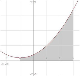
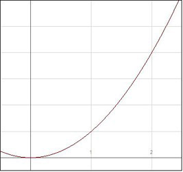
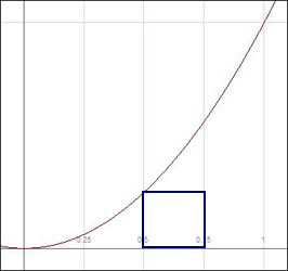
Let’s look at the function ![]() over the interval
over the interval ![]() . Suppose we wish to determine the area bounded by the curve and the x-axis, as depicted below.
. Suppose we wish to determine the area bounded by the curve and the x-axis, as depicted below.
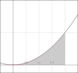
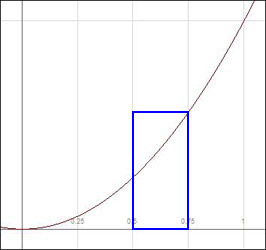
We can estimate the area under the curve by drawing rectangles over fixed intervals (in this case, intervals of ![]() ), with either the left corner or right corner of the rectangle’s upper width touching the curve, as depicted below.
), with either the left corner or right corner of the rectangle’s upper width touching the curve, as depicted below.
 |
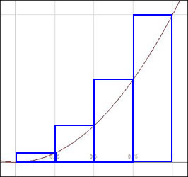 |
The area inside the rectangles is easy to compute. The area in the first graph is ![]() , while the area in the second graph is
, while the area in the second graph is ![]() . We know the actual area
. We know the actual area ![]() under the curve is between these two values, .22 and .47. We can narrow the range by taking smaller intervals, such as every
under the curve is between these two values, .22 and .47. We can narrow the range by taking smaller intervals, such as every ![]() .
.
We then compute the new areas ![]() and
and ![]() .
.
![]()
and
![]()
![]()
We still have not arrived at a good approximation of the area, but the interval width has narrowed from ![]() to
to ![]() . By continuing to narrow the intervals, both calculations will approximate the true area under the curve (which is
. By continuing to narrow the intervals, both calculations will approximate the true area under the curve (which is ![]() ) more and more closely.
) more and more closely.
This method of measuring the area as a series of rectangles is known as a Riemann sum. More specifically, the first graph is an example of a left Riemann sum, and the second graph is a right Riemann sum. The intervals, ![]() , for the two calculations are examples of partitions. In the first calculation, the right partition contains
, for the two calculations are examples of partitions. In the first calculation, the right partition contains ![]() subintervals of equal length. In the second calculation, the right partition contains
subintervals of equal length. In the second calculation, the right partition contains ![]() subintervals. For a function
subintervals. For a function ![]() , we represent a Riemann sum using the notation
, we represent a Riemann sum using the notation ![]() , where
, where ![]() represents the
represents the ![]() partition.
partition.
As the subintervals become smaller, ![]() , and the Riemann sum approaches the true area. In the closed interval
, and the Riemann sum approaches the true area. In the closed interval ![]() , we define the definite integral of the function
, we define the definite integral of the function ![]() as:
as:
![]()
We refer to ![]() as the lower limit and
as the lower limit and ![]() as the upper limit.
as the upper limit.
To be precise, the area under the curve ![]() in the interval
in the interval ![]() is not
is not ![]() if the value of
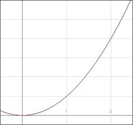
if the value of ![]() is negative in any part of the open interval. For example, look at the area under the curve
is negative in any part of the open interval. For example, look at the area under the curve ![]() on the interval
on the interval ![]() .
.
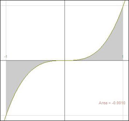
As we will see, if we were to evaluate the definite integral in the interval ![]() , we would find
, we would find ![]() , since the shaded area below the x-axis cancels out the symmetrically shaded area above the x-axis. To rectify this, we define the area as
, since the shaded area below the x-axis cancels out the symmetrically shaded area above the x-axis. To rectify this, we define the area as ![]() . In this example, we split the integral into two portions and find the sum of the positive values. Thus,
. In this example, we split the integral into two portions and find the sum of the positive values. Thus, ![]() .
.
In order to complete our understanding ![]() of definite integrals, we state and prove the Fundamental Theorem of Calculus.
of definite integrals, we state and prove the Fundamental Theorem of Calculus.
Let ![]() be a function continuous on
be a function continuous on ![]() and
and ![]() is any number in
is any number in ![]() .
.
(i) If we define ![]() , then
, then ![]() .
.
(ii) If we define ![]() , then
, then ![]() .
.
Proof of![]() :
:
Picture ![]() as the area under the curve
as the area under the curve ![]() from
from ![]() to
to ![]() . Then
. Then ![]() is the area from
is the area from ![]() to
to ![]() , and
, and ![]() is the area from
is the area from ![]() to
to ![]() . If
. If ![]() is small, the area from
is small, the area from ![]() to
to ![]() should be small. Also, since
should be small. Also, since ![]() is continuous,
is continuous, ![]() . That area should then approximate a rectangle of height
. That area should then approximate a rectangle of height ![]() and width
and width ![]() . Therefore,
. Therefore,
![]() , or
, or ![]() . As
. As ![]() , this approximation becomes exact, so
, this approximation becomes exact, so ![]()
![]() .
.
Proof of (![]() ):
):
Given ![]() , and using (i), it follows that
, and using (i), it follows that ![]() , which means
, which means ![]() ,or
,or ![]() . Therefore,
. Therefore, ![]() ,and
,and ![]() , so
, so ![]() . The second integral is clearly 0 (imagine the area of a rectangle with width 0). Therefore,
. The second integral is clearly 0 (imagine the area of a rectangle with width 0). Therefore, ![]() .
.
Part (ii) of the theorem states that the value of the definite integral on the interval ![]() is simply the difference of the antiderivative at the endpoints. Our shorthand is
is simply the difference of the antiderivative at the endpoints. Our shorthand is ![]() . Let’s try a couple of examples solving definite integrals.
. Let’s try a couple of examples solving definite integrals.
Find the actual areas under the curves on the given intervals:
(A) area under ![]() over the interval
over the interval ![]()
(B) area under ![]() over the interval
over the interval ![]()
(A) ![]() everywhere in the given interval, so
everywhere in the given interval, so ![]() .
.
(B) ![]() on the interval
on the interval ![]() , and
, and ![]() on the interval
on the interval ![]() , so
, so
![]()
A brick is dropped from the top of a building that is 500 meters tall. Its velocity after ![]() seconds is given by
seconds is given by ![]() meters per second. How long before the brick hits the ground?
meters per second. How long before the brick hits the ground?
You may recall that we found ![]() by taking the first derivative of the position
by taking the first derivative of the position ![]() ; that is,
; that is, ![]() . Here, we are given
. Here, we are given ![]() and need to solve for
and need to solve for ![]() , which is the antiderivative of the velocity function. From part (ii) of the Fundamental Theorem of Calculus, we know that
, which is the antiderivative of the velocity function. From part (ii) of the Fundamental Theorem of Calculus, we know that ![]() . In this example, a represents the time corresponding to the start of the fall and b represents the time corresponding to the end of the fall, the time we are looking for. So we will set
. In this example, a represents the time corresponding to the start of the fall and b represents the time corresponding to the end of the fall, the time we are looking for. So we will set ![]() seconds,
seconds, ![]() seconds, and solve for
seconds, and solve for ![]() . We know
. We know ![]() m and
m and ![]() . Therefore,
. Therefore, ![]() . Also, the total change in the brick’s position is simply its final position minus its initial position, or
. Also, the total change in the brick’s position is simply its final position minus its initial position, or ![]() meters. Therefore,
meters. Therefore, ![]() , or
, or ![]() seconds (
seconds (![]() ).
).
Before we proceed with the next example, let’s explore a notational detail which may seem strange at first. Recall that the expression ![]() can be read as, “G of x is the integral of f of x, with respect to x.” What if f(x) is a constant function? If f(x) = 5, then
can be read as, “G of x is the integral of f of x, with respect to x.” What if f(x) is a constant function? If f(x) = 5, then ![]() =
= ![]() . This can be read as, “G of x is 5 times the integral of 1, with respect to x.” We now know this is 5x + C, where C is some constant of integration. Typically, this last term is written in the simplified form
. This can be read as, “G of x is 5 times the integral of 1, with respect to x.” We now know this is 5x + C, where C is some constant of integration. Typically, this last term is written in the simplified form ![]() . If the integrand symbol followed by the dx with nothing in the middle seems strange, imagine a constant of 1 sitting between the integrand symbol and the dx.
. If the integrand symbol followed by the dx with nothing in the middle seems strange, imagine a constant of 1 sitting between the integrand symbol and the dx.
The marginal revenue (rate of change of revenue received per unit change in quantity sold) received by a retailer is given by ![]() , where
, where ![]() is the quantity of units sold. Compute the total revenue (
is the quantity of units sold. Compute the total revenue (![]() ) as a function of
) as a function of ![]() .
.
According to our definition of marginal revenue, ![]() . Therefore, we compute
. Therefore, we compute ![]() as the antiderivative of
as the antiderivative of ![]() .
.
![]()
To find a complete solution to the problem, we must now solve for C by checking to see what value of C will make our revenue function accurately reflect the conditions set forth in the original problem statement. If we sell a quantity of 0, we make no revenue.
![]() ,
,
or
![]() .
.
Our final solution is ![]() .
.
We’ve developed a formula for the area under the curve ![]() in
in ![]() :
: ![]() . More specifically, this formula describes the area under the curve
. More specifically, this formula describes the area under the curve ![]() bounded by the lines
bounded by the lines ![]() , and the x-axis. Let’s now consider the area bounded by two curves,
, and the x-axis. Let’s now consider the area bounded by two curves, ![]() and
and ![]() . Let
. Let ![]() , and
, and ![]() , and look at the area under each curve on
, and look at the area under each curve on ![]() .
.
 |
 |
The curves intersect at ![]() and
and ![]() , and their individual areas are represented by
, and their individual areas are represented by ![]() and
and ![]() .
.
Now let’s look at both graphs and the area between them on ![]() .
.
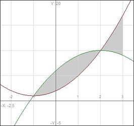
The area between the curves is the difference between the areas under each separate curve bounded by the x-axis. On ![]() ,
, ![]() , and the area is represented by
, and the area is represented by
![]()
On ![]() ,
, ![]() , and the area is
, and the area is
![]()
Therefore, to find the area ![]() on
on ![]() we need to solve the definite integrals.
we need to solve the definite integrals.
The area between two curves ![]() and
and ![]() , between
, between ![]() and
and ![]() is
is ![]() .
.
In some applications, it may be easier to compute the area of the region bounded by two curves by looking at horizontal elements rather than vertical rectangles. For example, look at the region bounded by the parabola ![]() and the line
and the line ![]() . The area of the region with a vertical rectangle is shown below.
. The area of the region with a vertical rectangle is shown below.

Note that the interval is on ![]() , and the line becomes the lower bound on
, and the line becomes the lower bound on ![]() . To compute the area this way, first, we need to solve the first equation for
. To compute the area this way, first, we need to solve the first equation for ![]() .
.
![]()
These separate equations represent the upper and lower halves of the parabola.
We solve for the total area in two parts. On ![]() , the integrand is the difference between the upper and lower halves of the parabola.
, the integrand is the difference between the upper and lower halves of the parabola.
![]()
On ![]() , the integrand is the difference between the upper half of the parabola and the line.
, the integrand is the difference between the upper half of the parabola and the line.
![]()
The total area is the sum ![]() .
.
Let’s look at this problem again, but this time, we will compute the area by taking horizontal rectangular elements. Note that the curves intersect at ![]() and
and ![]() .
.
First, we need to solve both equations for ![]() . We get
. We get ![]() and
and ![]() . The interval of integration is on the y-range
. The interval of integration is on the y-range ![]() , and the heights of the rectangles are
, and the heights of the rectangles are ![]() . Therefore, we can compute the total area between the curves with a single integral.
. Therefore, we can compute the total area between the curves with a single integral.
![]()
Clearly, this method is easier than the first.
Another application of definite integrals is calculating the volume of a solid of revolution. This is the solid created by revolving a portion of a curve about a line, such as the x– or y-axis. Let’s take ![]() on
on ![]() and see what happens if we revolve that portion of the curve about the x-axis and y-axis.
and see what happens if we revolve that portion of the curve about the x-axis and y-axis.
 |
 |
| x-axis | y-axis |
For the first graph, imagine a rectangular sliver of width ![]() as it revolves around the x-axis. It forms a circular disk of volume
as it revolves around the x-axis. It forms a circular disk of volume ![]() . We can approximate the volume as the sum of rectangles along the interval, just as we have been approximating the areas, but we will skip directly to what happens as
. We can approximate the volume as the sum of rectangles along the interval, just as we have been approximating the areas, but we will skip directly to what happens as ![]() . As
. As ![]() , the sum of rectangles becomes the definite integral on the interval
, the sum of rectangles becomes the definite integral on the interval ![]() , and the volume becomes
, and the volume becomes ![]() .
.
For example, solve ![]() .
.
Suppose we wish to revolve this same function on the same interval as in the second graph about the y-axis. First, we need to solve for ![]() . (In this case,
. (In this case, ![]() , as we are only looking at
, as we are only looking at ![]() .) Each sliver forms a disk of volume
.) Each sliver forms a disk of volume ![]() , and we integrate on the y-interval
, and we integrate on the y-interval ![]() . The volume of the solid revolved around the y-axis is
. The volume of the solid revolved around the y-axis is ![]() .
.
Finally, the volume of the solid of revolution bounded by two curves ![]() and
and ![]() is found by using reasoning similar to that which we have used with areas. If both functions are continuous and
is found by using reasoning similar to that which we have used with areas. If both functions are continuous and ![]() over
over ![]() , then the volume of the solid of revolution of the region bounded by
, then the volume of the solid of revolution of the region bounded by ![]() and
and ![]() about the x-axis is
about the x-axis is
![]()
Another computation it is useful to be able to find is the area of surface of revolution. The area of the surface of revolution obtained by rotating ![]() on
on ![]() about the x-axis is
about the x-axis is
![]()
The area of the surface of revolution obtained by rotating ![]() on the y-interval
on the y-interval ![]() about the y-axis is
about the y-axis is
![]()
Another application of definite integrals is finding the length of a curve, or arc length. You should recall that the distance between point ![]() and point
and point ![]() is
is ![]() . We can approximate the arc length of a curve continuous on
. We can approximate the arc length of a curve continuous on ![]() as the sum of straight lines between points
as the sum of straight lines between points ![]() and
and ![]() . Each small segment has a length
. Each small segment has a length  . As the length intervals become infinitesimally small, the exact length can be computed as the definite integral on
 ![]() . The value
. The value ![]() approaches
approaches ![]() (the proof of this utilizes the mean value theorem) and
(the proof of this utilizes the mean value theorem) and ![]() . As long as
. As long as ![]() and
and ![]() are continuous on
are continuous on ![]() , the length of the curve from
, the length of the curve from ![]() to
to ![]() is given by
is given by
![]()
If we want to find the length of the curve ![]() from
from ![]() to
to ![]() and
and ![]() and
and ![]() are continuous on
are continuous on ![]() , the length of the curve is
, the length of the curve is
![]()
The final application of definite integrals we will examine is the work done by a force acting on an object. If the object is acted on by a force ![]() and is displaced along the x-axis from point
and is displaced along the x-axis from point ![]() to point
to point ![]() , the work done by the force is
, the work done by the force is ![]() . Work is usually measured in foot-pounds, or, if the force is in newtons and the displacement is in meters, in joules. Sometimes, force is measured in dynes and displacement in centimeters. Then, work is measured in dyne-cm, or ergs.
. Work is usually measured in foot-pounds, or, if the force is in newtons and the displacement is in meters, in joules. Sometimes, force is measured in dynes and displacement in centimeters. Then, work is measured in dyne-cm, or ergs.
Let’s try an example. Consider the curve ![]() from
from ![]() to
to ![]() . Compute the following:
. Compute the following:
(A) the area under the curve bounded by the x-axis, using vertical rectangles;
(B) the area under the curve bounded by the x-axis, using horizontal rectangular elements;
(C) the volume of the solid of revolution about the x-axis; and
(D) the volume of the solid of revolution about the y-axis.
(A) ![]()
(B) Solve ![]() for x.
for x. ![]() . At
. At ![]() , and at
, and at ![]() . The height of each rectangle is
. The height of each rectangle is ![]() , and its width is
, and its width is ![]() . Therefore,
. Therefore,

(C) ![]()
(D) ![]()
Let’s try a second example. For the line ![]() , find:
, find:
(A) the length of arc from ![]() to
to ![]() ; and
; and
(B) the area of surface of revolution about the x-axis over the same interval.
(A) At ![]() ,
, ![]() ; at
; at ![]() ,
, ![]() . Also,
. Also, ![]() , so
, so ![]() . Therefore,
. Therefore,
Since the curve in question is simply a line, we can verify this solution by using the distance formula to find the distance between the points (9, 7) and (18, 10). Indeed, the distance formula gives us the same answer for the length of the arc from ![]() to
to ![]() .
.
So far, we have solved definite and indefinite integrals where the integrand is of the form ![]() ,
, ![]() , and
, and ![]() . This section examines integrals of various functions, and techniques for solving integrals of various forms.
. This section examines integrals of various functions, and techniques for solving integrals of various forms.
The first method we will examine is integration by substitution. We know how to solve for integrals in the form ![]() (
(![]() ). For example, we know how to solve
). For example, we know how to solve ![]() . This method does not work if the power of
. This method does not work if the power of ![]()
![]() . However, we can use substitution to solve a similar integral:
. However, we can use substitution to solve a similar integral: ![]() . Let
. Let ![]() , so
, so ![]() and substitute
and substitute ![]() for
for ![]() .
.
Thus, if we have an integral whose integrand can be placed in the form ![]()
![]() , we can use the chain rule and substitution to transform the integral to the form
, we can use the chain rule and substitution to transform the integral to the form ![]() . Then, it can be easily integrated.
. Then, it can be easily integrated.
For the case ![]() , we can determine
, we can determine ![]() . Recall from differential calculus that
. Recall from differential calculus that ![]() . But
. But ![]() . Therefore,
. Therefore,
![]()
Let’s try a few examples. Compute ![]() .
.
Let ![]() . Then
. Then ![]() . Therefore,
. Therefore,
![]()
Compute ![]() . Let
. Let ![]() , and
, and ![]() . Therefore
. Therefore
![]()
What is integration by parts?
Another integration technique is known as integration by parts. If an integral is in the form ![]() , but can be solved in the form
, but can be solved in the form ![]() , use the following.
, use the following.
![]()
This formula is derived from the product rule in differential calculus. Recall that ![]() . When solving for
. When solving for ![]() , we find that
, we find that ![]() . Finally, integrate all three terms to arrive at the formula. The goal of integration by parts is to transform one integral into another integral that is “solvable.” After deciding what to call
. Finally, integrate all three terms to arrive at the formula. The goal of integration by parts is to transform one integral into another integral that is “solvable.” After deciding what to call ![]() and
and ![]() and solving for
and solving for ![]() and
and ![]() , one of three things should happen:
, one of three things should happen:
(1)![]() is as hard or harder to solve than
is as hard or harder to solve than ![]() , and the process is abandoned.
, and the process is abandoned.
(2) ![]() is easy to solve, and the formula is straightforward.
is easy to solve, and the formula is straightforward.
(3) Solving for ![]() leads to a solution with
leads to a solution with ![]() , which is solved by algebra.
, which is solved by algebra.
The following examples illustrate each of these scenarios.
Compute ![]() by setting
by setting ![]() and
and ![]() .
.
We find that ![]() Therefore,
Therefore, ![]() However, this new integral is even more difficult to solve than the original, so we abandon this process.
However, this new integral is even more difficult to solve than the original, so we abandon this process.
Compute ![]() by setting
by setting ![]() and
and ![]() .
.
We find that ![]() . Therefore,
. Therefore, ![]() . We can easily solve this new integral by substitution. Let
. We can easily solve this new integral by substitution. Let ![]() , so
, so ![]() . The integral is
. The integral is ![]() . So,
. So,
![]()
These first two examples illustrate an important point about integration problems and the methods used. For most of our mathematical career, mathematics is generally algorithmic. As long as rules and procedures are memorized and practiced, a solution can usually be reached through careful perseverance. This is not the case when working with integrals. In fact, the integrals of most functions, if they are randomly drawn from the “universe of functions,” are not solvable manually by any of our methods. Even if they are solvable, not every possible method will get us to the solution. Don’t let this frustrate you, and try to remember that with practice, you will begin to recognize patterns in the structure of the functions you are integrating which give clues as to possible methods that might be worth trying.
Compute ![]() .
.
First, let ![]() . Set
. Set ![]() , and
, and ![]() . We find that
. We find that ![]() . Therefore,
. Therefore, ![]() To solve this new integral, perform integration by parts. Set
To solve this new integral, perform integration by parts. Set ![]() and
and ![]() . It is then true that
. It is then true that ![]() , so
, so ![]()
![]() . Now, we have
. Now, we have ![]() If we apply simple algebra, we find that
If we apply simple algebra, we find that ![]() or
or ![]() . Therefore,
. Therefore,
![]()
If the integrand is in the form ![]() , we can solve the integral by trigonometric substitution. Recall the trigonometric identities
, we can solve the integral by trigonometric substitution. Recall the trigonometric identities ![]() and
and ![]() . If we set
. If we set ![]() , the term
, the term ![]() simplifies to
simplifies to ![]() If we set
If we set ![]() , the term
, the term ![]() simplifies to
simplifies to ![]()
![]() . And if we set
. And if we set ![]() , the term
, the term ![]() simplifies to
simplifies to ![]()
Trigonometric substitution is often easier with definite integrals than with indefinite integrals. With definite integrals, we can leave the answer in terms of ![]() and change the upper and lower limit of the integral into terms of
and change the upper and lower limit of the integral into terms of ![]() rather than
rather than ![]() , where appropriate. With indefinite integrals, we must change
, where appropriate. With indefinite integrals, we must change ![]() to
to ![]() , which can be tricky. Let’s try an example. Compute
, which can be tricky. Let’s try an example. Compute  . Hint:
 ![]() .
.
Let ![]() , so
, so ![]() . Since the 0 and 1 correspond to x-values, not θ-values, we must change the limits of integration. Since
. Since the 0 and 1 correspond to x-values, not θ-values, we must change the limits of integration. Since ![]() , and we are now integrating with respect to θ, we look for a θ value which will make sin θ = 0. This requirement is met when θ = 0. The new upper limit, which corresponds to
, and we are now integrating with respect to θ, we look for a θ value which will make sin θ = 0. This requirement is met when θ = 0. The new upper limit, which corresponds to ![]() , is satisfied when
, is satisfied when ![]() , or
, or ![]() . Therefore,
. Therefore,
The next integration technique is useful when the integrand can be expressed as a rational function, that is, the quotient of two polynomial functions ![]() . This method involves breaking up
. This method involves breaking up ![]() into the sum of partial fractions. For example, if the integrand is
into the sum of partial fractions. For example, if the integrand is ![]() , create partial fractions by setting
, create partial fractions by setting ![]() . By rewriting each term on the right so that the denominators are identical to the denominator on the left and reducing, we have
. By rewriting each term on the right so that the denominators are identical to the denominator on the left and reducing, we have ![]() Factoring and rearranging terms gives
Factoring and rearranging terms gives ![]() We now have 3 equations and 3 unknowns
We now have 3 equations and 3 unknowns ![]() . The solution you should get is
. The solution you should get is ![]() . We can use these terms to rewrite the integrand as the sum of three simple terms and integrate each one separately.
. We can use these terms to rewrite the integrand as the sum of three simple terms and integrate each one separately.
Here is another example. Compute ![]() .
.
Using partial fractions, we rewrite this integral as
When the denominator has factors in the form ![]() for
for ![]() , all factors of
, all factors of ![]() must be included in partial fractions. For example, the quotient
must be included in partial fractions. For example, the quotient ![]() is broken up into partial fractions
is broken up into partial fractions ![]() .
.
Another technique involving rational functions is completing the square. This technique is illustrated in the following example.
Compute ![]() by completing the square.
by completing the square.

Set ![]() , so
, so ![]() . Therefore,
. Therefore,
We solve this integral by partial fractions:
![]() .
.
Therefore, ![]()
The solution is ![]() , so
, so
![]()
The next form of function requires an understanding of inverse trigonometric functions. For example, the inverse sine function ![]() is satisfied if
is satisfied if ![]() . We know
. We know ![]() is in the interval
is in the interval ![]() . In order for each value of x in this interval to have a unique
. In order for each value of x in this interval to have a unique ![]() , we restrict
, we restrict ![]() to the interval
to the interval  . The inverse cosine function
 ![]() exists if and only if
exists if and only if ![]() on
on ![]() . The inverse tangent function
. The inverse tangent function ![]() exists if and only if
exists if and only if ![]() on
on  . The inverse secant function
From the formulas for the derivatives of the inverse trigonometric functions, we obtain the following indefinite integrals.

Techniques such as substitution and completing the square are often required in order to factor the integrand into one of the above forms.
Using the integration techniques introduced in this module along with other techniques and tricks, we are capable of integrating and, in the case of definite integrals, finding an exact numerical solution. Unfortunately, exact solutions cannot be found for all definite integrals, such as  and
and  . For these circumstances, we rely on methods of numerical or approximate integration. We already examined a method of approximating the value of a definite integral: the Riemann sum. However, the example we looked at demonstrates that this is a slow-converging approximation method. We will now examine two numerical methods that provide better accuracy: the trapezoidal rule and Simpson’s rule.
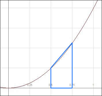
With Riemann sums, the area of each subinterval is approximated as a rectangle along the partition. The trapezoidal rule more accurately defines each area as a trapezoid, which better represents the change in the function. We illustrate this point by referring back to our original function, ![]() . Compare the areas on the interval
. Compare the areas on the interval ![]() of a left Riemann sum, right Riemann sum, and trapezoid with the exact area
of a left Riemann sum, right Riemann sum, and trapezoid with the exact area  .
.
 |
 |
 |
|
Area
under a curve 1 |
Area
under curve 2 |
Area
under curve 3 |
The area of the first region is ![]() . The area of the second region is
. The area of the second region is ![]() . The area of the third region is
. The area of the third region is ![]() . The true area is
. The true area is 
![]() .
.
Clearly, the trapezoid is closer to the true area than either rectangle. (The trapezoidal area is actually the average of ![]() .)
.)
If ![]() is continuous on
is continuous on ![]() and
and ![]() are regular partitions of
are regular partitions of ![]() , then the trapezoidal rule states:
, then the trapezoidal rule states:
Now use the trapezoidal rule to estimate the area under the curve ![]() with
with ![]() .
.
This is the same interval we examined previously. Recall that we determined ![]() using Riemann sums. First, compute
using Riemann sums. First, compute ![]() . Therefore,
. Therefore,
![]()
The trapezoid formula converges to the true area ![]() with 8 intervals more efficiently than either Riemann sum.
with 8 intervals more efficiently than either Riemann sum.
The trapezoidal rule, like Riemann sums, approximates the definite integral as the sum of areas formed by straight lines connecting two points. In contrast, Simpson’s rule computes the area bounded by parabolas connecting three points. This gives us a better approximation to the area under the curve. Simpson’s rule states:

Note that Simpson’s rule has ![]() subintervals while the trapezoid rule has
subintervals while the trapezoid rule has ![]() subintervals.
subintervals.
For example, use Simpson’s rule to compute  with
with ![]() .
.
![]()
= ![]()
The reason this value is the exact area is that Simpson’s rule assumes each partition is a parabola, and in this case, ![]() is an actual parabola.
is an actual parabola.
We conclude our analysis of integral calculus with improper integrals. This is a type of definite integral  where either
 ![]() , or
, or ![]() becomes infinite for some value of
becomes infinite for some value of ![]() on
on ![]() .
.
Provided that ![]() is continuous on the interval defined by the lower and upper limits of the integral, the following rules apply.
is continuous on the interval defined by the lower and upper limits of the integral, the following rules apply.
![]()
for some real number ![]()
If the limit exists and is finite, the improper integral is convergent. If the improper integral does not exist, it is divergent. The integral diverges if it blows up to ![]() , or if it has no defined limit. An example of the latter situation is
, or if it has no defined limit. An example of the latter situation is  .
.
Compute the area bounded by the x-axis on ![]() for the following curves:
for the following curves:
(A)![]() ; and
; and
(B)![]() .
.
(A) .
.
(B) .
.
This limit does not exist—it blows up to ![]() . This improper integral is divergent.
. This improper integral is divergent.
Another type of improper integral is one that blows up at one or more points on a finite interval. Such a point is represented by a vertical asymptote. If ![]() has a vertical asymptote on
has a vertical asymptote on ![]() at
at ![]() , and if
, and if  exist for
 ![]() in
in ![]() , and for
, and for ![]() in
in ![]() , then
, then
Compute  .
.
The integrand has an infinite discontinuity at ![]() , as illustrated below
, as illustrated below
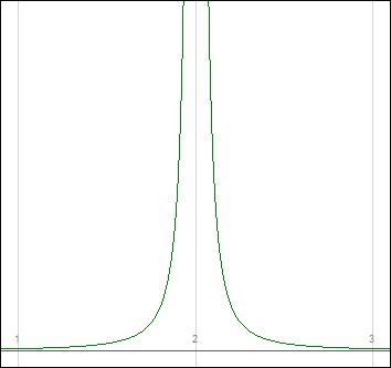
Applying the above rule to this integral, with ![]() , we find
, we find
Since neither of these limits exists, the integral is divergent. Had we not recognized the discontinuity and attempted to solve the definite integral, we would have arrived at the wrong answer of ![]() . This answer makes no sense, since the integrand is always positive.
. This answer makes no sense, since the integrand is always positive.