In this lesson, you will cover the definition of a derivative and apply it to the evaluation of slopes and tangent lines of curves, instantaneous rates of changes of functions, relative maxima and minima, and methods to compute the derivative of several types of functions.
Up to this point, we have differentiated functions defined as ![]() . In other words,
. In other words, ![]() is defined explicitly in terms of the variable
is defined explicitly in terms of the variable ![]() . There are situations where we define
. There are situations where we define ![]() in terms of a third variable, or parameter, such as
in terms of a third variable, or parameter, such as ![]() . In order to find
. In order to find ![]() , we apply parametric differentiation. Similarly, we may have an equation (not necessarily a function) that relates
, we apply parametric differentiation. Similarly, we may have an equation (not necessarily a function) that relates ![]() , but is not in the form
, but is not in the form ![]() . An example is the equation of a circle with a radius
. An example is the equation of a circle with a radius ![]() , centered about the origin:
, centered about the origin: ![]() . We find
. We find ![]() through a similar technique known as implicit differentiation.
through a similar technique known as implicit differentiation.
The rule for parametric differentiation is simple:
If ![]() , we can find
, we can find ![]() by solving the ratio
by solving the ratio  , where
 ![]() .
.
This is actually a consequence of the chain rule.
For example, suppose x = t3 + 4t – 1, and y = 6 – t2. Use parametric differentiation to find ![]() .
.
If we were to solve this using only the tools we had in the last section, we would have to find a formula for ![]() in terms of
in terms of ![]() (which may be next to impossible) and substitute that formula into the equation for
(which may be next to impossible) and substitute that formula into the equation for ![]() , so we would be left with an expression for
, so we would be left with an expression for ![]() .
.
However, parametric differentiation makes this much easier:
![]() .
.
If, as in this case, the formula for ![]() cannot easily be defined in terms of
cannot easily be defined in terms of ![]() , you can create a table of values for
, you can create a table of values for ![]() .
.
This should provide information on the relationship of ![]() to
to ![]() . Some problems simply provide the
. Some problems simply provide the ![]() value.
value.
Given the equation of a circle, ![]() , with constant radius
, with constant radius ![]() , use implicit differentiation to solve for
, use implicit differentiation to solve for ![]() .
.
Without implicit differentiation, we can solve for y.
![]()
We have two separate functions, one for the top semicircle, and the other for the bottom semicircle. We can then use the chain rule to solve for both values of ![]() .
.
Now we will examine how to use implicit differentiation. First, since both sides of the equation are equal, their derivatives are equal. Also, recall that the derivative of the left side of the equation is the same as the derivative of each of the two terms. To find ![]() , we will take the derivative
, we will take the derivative ![]() of all three terms.
of all three terms.
![]()
Therefore, ![]() . (The second term uses the chain rule since y is indeed dependent upon x, and the third term is
. (The second term uses the chain rule since y is indeed dependent upon x, and the third term is ![]() because
because ![]() is a constant with respect to x).
is a constant with respect to x).
![]()
We actually have two solutions for ![]() , depending on whether we are interested in the upper or lower semicircle.
, depending on whether we are interested in the upper or lower semicircle.
![]()
The first equation describes the slope of the upper semicircle of a circle of radius ![]() centered about the origin, while the second equation describes the slope of the lower semicircle.
centered about the origin, while the second equation describes the slope of the lower semicircle.
Using the tools of implicit differentiation, we are able to use differential calculus for applications known as related rates of change. We will solve two classic related rates problems: the sliding ladder and the leaking container.
A 10-foot ladder is leaning at an angle against a wall, with the foot of the ladder on the floor. The foot of the ladder is sliding across the floor at a rate of ![]() feet per second. When the foot of the ladder is
feet per second. When the foot of the ladder is ![]() feet from the wall, how fast is the top of the ladder sliding down the wall?
feet from the wall, how fast is the top of the ladder sliding down the wall?
The wall, floor, and ladder form a right triangle, so we will use the Pythagorean Theorem to solve. The equation is ![]() , where
, where ![]() is the distance from the wall to the foot of the ladder,
is the distance from the wall to the foot of the ladder, ![]() is the height from the floor to the top of the ladder, and
is the height from the floor to the top of the ladder, and ![]() is the length of the ladder, which we know is 10 feet. We are asked to find the rate at which the top of the ladder is sliding down the wall, which according to our choice of variables is equivalent to
is the length of the ladder, which we know is 10 feet. We are asked to find the rate at which the top of the ladder is sliding down the wall, which according to our choice of variables is equivalent to ![]() . Be careful when you approach problems such as this, as we could have been asked to find the rate at which the bottom of the ladder is sliding across the floor. In that case we would be looking for
. Be careful when you approach problems such as this, as we could have been asked to find the rate at which the bottom of the ladder is sliding across the floor. In that case we would be looking for ![]() . Since we are interested in changing rates over time, we take
. Since we are interested in changing rates over time, we take ![]() of all terms.
of all terms.
![]()
Therefore, ![]() .
.
At the beginning of this problem, we identified that we are looking for ![]() , so we will use this equation, and isolate that particular term. Solving for
, so we will use this equation, and isolate that particular term. Solving for ![]() ,
, ![]() . We are given
. We are given ![]() , and
, and ![]() feet per second. We still need to find the value of
feet per second. We still need to find the value of ![]() . That can be determined by using the Pythagorean Theorem again.
. That can be determined by using the Pythagorean Theorem again. ![]() , which gives us
, which gives us ![]() feet as the only positive answer. Therefore,
feet as the only positive answer. Therefore, ![]() feet per second. Note that the answer is negative, since the ladder is sliding in the
feet per second. Note that the answer is negative, since the ladder is sliding in the ![]() direction.
direction.
A paper cup in the shape of a right circular cone has a height of ![]() inches and a radius of
inches and a radius of ![]() inches at its rim. It is filled with water, but develops a leak out of the bottom, at a rate of 0.1 cubic inch per minute. At what rate is the height of the water dropping when the cup is filled to a height of 3 inches?
inches at its rim. It is filled with water, but develops a leak out of the bottom, at a rate of 0.1 cubic inch per minute. At what rate is the height of the water dropping when the cup is filled to a height of 3 inches?
In order to solve this problem, you need to know that the volume of a right circular cone is ![]() , and, according to the law of similar triangles, the ratio
, and, according to the law of similar triangles, the ratio ![]() is constant at all heights. From this, we eliminate
is constant at all heights. From this, we eliminate ![]() in the volume equation.
in the volume equation.
We are given ![]() and need to solve for
and need to solve for ![]() , or the rate at which the height of the water is changing with respect to time. The first sentence tells us
, or the rate at which the height of the water is changing with respect to time. The first sentence tells us ![]() , so
, so ![]() . Therefore,
. Therefore, ![]() . Taking
. Taking ![]() of both sides, we find
of both sides, we find
![]() , or
, or ![]()
We are given ![]() and
and ![]() . Therefore,
. Therefore, ![]() inches per minute.
inches per minute.
The derivative ![]() is known as a first derivative of
is known as a first derivative of ![]() , or the first derived function. A derivative of a derivative is known as a second derivative function. One way a second derivative is denoted is
, or the first derived function. A derivative of a derivative is known as a second derivative function. One way a second derivative is denoted is ![]() , which is read, “
, which is read, “![]() double prime.” We actually computed a second derivative earlier, when we calculated the acceleration in the example of a moving particle.
double prime.” We actually computed a second derivative earlier, when we calculated the acceleration in the example of a moving particle.
Recall that we found the velocity ![]() by taking the derivative of the position
by taking the derivative of the position ![]() :
: ![]() , and then found the acceleration g by taking the derivative of the velocity,
, and then found the acceleration g by taking the derivative of the velocity, ![]() . We see that
. We see that ![]() .
.
Another way to write the second derivative function is
![]()
Typically, third derivative functions also use primes, such as ![]() . Beyond that, we typically put the order in parentheses, like this:
. Beyond that, we typically put the order in parentheses, like this: ![]() .
.
Alternatively, we can use the notation ![]() , which does not use parentheses. Power functions may eventually reach a point where higher-order derivatives are all zero. Other functions, like trigonometric, logarithmic, and exponential functions, can have infinite orders of derivatives.
, which does not use parentheses. Power functions may eventually reach a point where higher-order derivatives are all zero. Other functions, like trigonometric, logarithmic, and exponential functions, can have infinite orders of derivatives.
Let’s try an example. Compute all higher order derivatives of ![]() (until
(until ![]() ).
).

Let’s try another example. Let ![]() . Compute
. Compute ![]() , and extrapolate an equation for
, and extrapolate an equation for ![]() .
.
To solve, rewrite ![]() .
.

Note that the higher order derivatives alternate between + and – . You may also notice another pattern — the ![]() order derivative has
order derivative has ![]() in the numerator and
in the numerator and ![]() in the denominator. The alternating signs can be mathematically represented as
in the denominator. The alternating signs can be mathematically represented as ![]() . Therefore, the
. Therefore, the ![]() derivative of y is
derivative of y is ![]() .
.
Try one final example. Given ![]() , compute
, compute ![]() .
.
We are being asked to find the second derivative of y, with respect to x. We need to use implicit differentiation, the chain rule, and the quotient rule to solve this problem.
First, find ![]() by taking
by taking ![]() of each term.
of each term.
![]()
Next, solve for ![]() .
.
![]()
Next, substitute the value of ![]() into the above equation.
into the above equation.
Finally, notice that due to some careful algebra, we have managed to write this last quantity in such a way that it contains the term ![]() . We know from the original problem statement that this term has a specific numerical value of 16 for that expression. When solving implicit differentiation problems on your own, look carefully for opportunities to use initial information like this. We now substitute
. We know from the original problem statement that this term has a specific numerical value of 16 for that expression. When solving implicit differentiation problems on your own, look carefully for opportunities to use initial information like this. We now substitute ![]() for the value of
for the value of ![]() .
.
![]()
Before we proceed, we will define other key derivatives without proof. We are going to assume the reader is familiar with natural logarithms and exponential functions, as well as their properties.
If we know the derivative of ![]() , we can find the derivatives of other trigonometric functions. For example, it is easy to prove
, we can find the derivatives of other trigonometric functions. For example, it is easy to prove ![]() . Simply write
. Simply write ![]() , differentiate using the quotient rule, and utilize the trigonometric identity
, differentiate using the quotient rule, and utilize the trigonometric identity ![]() .
.
The following are important derivatives to know:

Do not forget that the chain rule can apply to any function. For example, ![]() . Derivatives for inverse trigonometric functions (e.g.
. Derivatives for inverse trigonometric functions (e.g. ![]() ) and hyperbolic trigonometric functions (e.g.
) and hyperbolic trigonometric functions (e.g. ![]() ) are beyond the scope of this module, but can be found in many calculus textbooks, math formula books, and are often provided as references when taking tests.
) are beyond the scope of this module, but can be found in many calculus textbooks, math formula books, and are often provided as references when taking tests.
Two interesting rules apply in differential calculus when a function is continuous and differentiable on an interval. The first is Rolle’s Theorem.
Let ![]() be a function such that:
be a function such that:
Then there is at least one number ![]() in (a, b) such that
in (a, b) such that ![]() .
.
Of course, this is obvious if ![]() for all
for all ![]() in
in ![]() . Since
. Since ![]() for all
for all ![]() , any number
, any number ![]() in
in ![]() will satisfy
will satisfy ![]() .
.
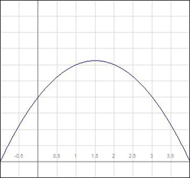
We will illustrate Rolle’s Theorem with the graph ![]() (
( ![]() in degrees), on the interval
in degrees), on the interval ![]() and the interval
and the interval ![]() . This function is both continuous and differentiable for all
. This function is both continuous and differentiable for all ![]() .
.
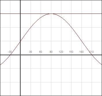
In the first graph, ![]() in the interval for
in the interval for ![]() and
and ![]() . According to Rolle’s Theorem, there must be at least one point in the interval
. According to Rolle’s Theorem, there must be at least one point in the interval ![]() where
where ![]() . That point is
. That point is ![]() .
.

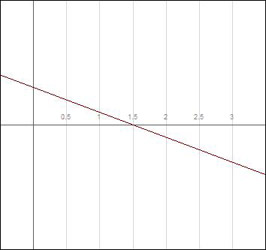
In the second graph, ![]() in the interval for
in the interval for ![]() and
and ![]() . According to Rolle’s Theorem, there must be at least one point in the interval
. According to Rolle’s Theorem, there must be at least one point in the interval ![]() where
where ![]() . That point is
. That point is ![]() .
.
Now we can make a couple of observations about this graph. First, the line tangent to the point at which ![]() is always parallel to the x-axis. Second, the points at which
is always parallel to the x-axis. Second, the points at which ![]() appear to define some type of maximum or minimum of the curve in an interval. We will be discussing this second observation in great detail later.
appear to define some type of maximum or minimum of the curve in an interval. We will be discussing this second observation in great detail later.
Let’s try an example. The position of a ball thrown up in the air from the ground is described by the equation ![]() ,
,
where ![]() is the upward velocity at
is the upward velocity at ![]() , and
, and ![]() is the downward acceleration due to gravity
is the downward acceleration due to gravity
(![]() are constant). At some time
are constant). At some time ![]() , the ball will strike the ground. Use Rolle’s Theorem to prove that, at some time
, the ball will strike the ground. Use Rolle’s Theorem to prove that, at some time ![]() , the velocity of the ball will be exactly 0.
, the velocity of the ball will be exactly 0.
You know from experience that when you throw a ball in the air, the position ![]() and velocity
and velocity ![]() of the ball do not abruptly change at any time. Therefore,
of the ball do not abruptly change at any time. Therefore, ![]() is continuous and differentiable. Also, we are given
is continuous and differentiable. Also, we are given ![]() . Since all three conditions for Rolle’s Theorem are met, we know there is some time
. Since all three conditions for Rolle’s Theorem are met, we know there is some time ![]() in the interval
in the interval ![]() where
where ![]() . This time is when the ball reaches its peak height before coming back down.
. This time is when the ball reaches its peak height before coming back down.
Rolle’s Theorem is used to prove a very important rule in calculus known as the Mean Value Theorem.
Let ![]() be continuous on the closed interval
be continuous on the closed interval ![]() and differentiable on the open interval
and differentiable on the open interval ![]() . Then there exists at least one number
. Then there exists at least one number ![]() in the open interval
in the open interval ![]() such that
such that ![]() .
.
You may recall that we saw an equation similar to this when we interpreted the derivative in terms of a tangent line. It is the formula for the slope of the secant line connecting the points ![]() on the
on the ![]() curve. We also know that
curve. We also know that ![]() is the slope of the curve at
is the slope of the curve at ![]() . Therefore, this theorem simply states that, for any secant line drawn on a curve, there is at least one point in between at which the tangent line is parallel to the secant line.
. Therefore, this theorem simply states that, for any secant line drawn on a curve, there is at least one point in between at which the tangent line is parallel to the secant line.

Since this curve meets the continuity and differentiability rules of the Mean Value Theorem, the point ![]() must exist somewhere in the
must exist somewhere in the ![]() interval.
interval.
Given the function ![]() over the interval
over the interval ![]() , what is the value of
, what is the value of ![]() that satisfies the Mean Value Theorem?
that satisfies the Mean Value Theorem?
The correct choice is D. If we were to try to find ![]() whereby
whereby ![]() , we would first compute
, we would first compute ![]() and
and ![]() . Therefore,
. Therefore,  . We compute
 ![]() , so we need to find
, so we need to find ![]() such that
such that ![]() . This is true when
. This is true when ![]() , which has no real solutions.
, which has no real solutions.
You might think that this example implies that the Mean Value Theorem is incorrect. However, this is not the case. Remember that ![]() must be continuous and differentiable in the interval
must be continuous and differentiable in the interval ![]() , and
, and ![]() is neither continuous nor differentiable at
is neither continuous nor differentiable at ![]() , which is in the open interval. Therefore, the Mean Value Theorem does not apply here.
, which is in the open interval. Therefore, the Mean Value Theorem does not apply here.
When discussing how to determine limits in the previous module, we mentioned that there was a way to determine the limits of quotients in the form ![]() , which reduce to
, which reduce to ![]() . This is known as L’Hôpital’s rule. There are two versions of this rule; the first is for the situation in which we find the limit of the quotient as
. This is known as L’Hôpital’s rule. There are two versions of this rule; the first is for the situation in which we find the limit of the quotient as ![]() , and the second for the situation in which we find the limit of the quotient as
, and the second for the situation in which we find the limit of the quotient as ![]() .
.
L’Hôpital’s rule for the indeterminate form ![]() :
:
If ![]() are functions that are differentiable for in an interval around
are functions that are differentiable for in an interval around ![]() (except possibly at
(except possibly at ![]() ), and both
), and both ![]() and
and ![]() , then if
, then if ![]() , where
, where ![]() is a real number or ,
is a real number or , ![]() then
then ![]() .
.
L’Hôpital’s rule for the indeterminate form ![]() :
:
If ![]() are functions that are differentiable for in an interval around
are functions that are differentiable for in an interval around ![]() (except possibly at
(except possibly at ![]() ), and both
), and both ![]() and
and ![]() , then if
, then if ![]() , where
, where ![]() is a real number or ,
is a real number or , ![]() then
then ![]()
When written out formally, this rule sounds much more complicated than it really is. L’Hôpital’s rule is a method used to compute the limit of a function in which the variable is in the numerator and denominator. If plugging the value of the limit that ![]() approaches into the function leads to either
approaches into the function leads to either ![]() , then just take the derivative of the numerator and the derivative of the denominator. Check out this new ratio. If you still get,
, then just take the derivative of the numerator and the derivative of the denominator. Check out this new ratio. If you still get, ![]() , take the derivative again. Finally, whatever number you get as the limit, is the limit for the original function.
, take the derivative again. Finally, whatever number you get as the limit, is the limit for the original function.
You can only use L’Hôpital’s rule whenever the limit is ![]() . Applying this rule to any finite, nonzero limit will produce an erroneous result.
. Applying this rule to any finite, nonzero limit will produce an erroneous result.
Let’s try an example. Use L’Hôpital’s rule to prove the trigonometric limits that you were previously asked to memorize:
(A) ![]() ; and
; and
(B) ![]() .
.
(A) First, note that ![]() , so we know we can apply this rule.
, so we know we can apply this rule.
The derivative of the numerator is ![]() , and the derivative of the denominator is
, and the derivative of the denominator is ![]() . Therefore,
. Therefore,
![]() .
.
(B) First, note that ![]() , so we know that we can apply this rule again. The derivative of the numerator is
, so we know that we can apply this rule again. The derivative of the numerator is ![]() , and the derivative of the denominator is
, and the derivative of the denominator is ![]() . Therefore,
. Therefore,
![]()
Let’s try a second example. Find ![]() .
.
By plugging in ![]() , you should find that both the numerator and denominator are 0 (
, you should find that both the numerator and denominator are 0 (![]() ). Therefore, take the derivative of the numerator and denominator.
). Therefore, take the derivative of the numerator and denominator.
![]()
Again, plugging in ![]() leaves us with
leaves us with ![]() . Therefore, take the derivatives again.
. Therefore, take the derivatives again.
![]()
Therefore, ![]() .
.
Let’s try one more example. Find ![]() .
.
First, note that the numerator and denominator both approach infinity as ![]() approaches infinity, so we have the indeterminate form
approaches infinity, so we have the indeterminate form ![]() . If we apply L’Hôpital’s rule, we find that
. If we apply L’Hôpital’s rule, we find that ![]() . Note that the second term in the denominator approaches 0 at the limit, but the numerator and denominator still results in
. Note that the second term in the denominator approaches 0 at the limit, but the numerator and denominator still results in ![]() .
.
This means it is necessary to take derivatives again. You should see a pattern: the numerator will always be ![]() , the first term of the denominator will always have a power function that will go down by one, and the second term in the denominator will always approach zero as
, the first term of the denominator will always have a power function that will go down by one, and the second term in the denominator will always approach zero as ![]() . Rather than take
. Rather than take ![]() derivatives before the first term in the denominator fails to approach
derivatives before the first term in the denominator fails to approach ![]() , you should see that the numerator will eventually win, so
, you should see that the numerator will eventually win, so ![]() . The end result is that
. The end result is that ![]() blows up more rapidly as
blows up more rapidly as ![]() than the
than the ![]() and
and ![]() functions combined.
functions combined.
In previous sections, we have applied differential calculus to determine slopes of tangent lines and rates of change of functions. We will now introduce other useful applications. First, we will use differentiation as a tool for curve sketching.
From what we know about derivatives, we can look at the graph of a function and roughly determine its slope at all points. Wherever the curve’s y-value increases with increasing ![]() , we know its slope (hence its derivative) is positive. The steeper the climb, the larger the value of the derivative in that interval.
, we know its slope (hence its derivative) is positive. The steeper the climb, the larger the value of the derivative in that interval.
Likewise, a curve that decreases in an interval will have a negative derivative. At a point where a curve changes direction, the derivative is zero. We will illustrate this point in the following example.
For what values of ![]() is the function
is the function ![]() increasing and decreasing? Determine this by (A) computing
increasing and decreasing? Determine this by (A) computing ![]() , and (B) sketching the curve
, and (B) sketching the curve ![]() .
.
(A) ![]() . The curve
. The curve ![]() increases in value whenever
increases in value whenever ![]() . Likewise, the curve decreases for all
. Likewise, the curve decreases for all ![]() .
.
(B) The curve for ![]() is depicted below.
is depicted below.

The curve clearly shows a parabola that decreases in value until ![]() , after which it increases. Note also that, at
, after which it increases. Note also that, at ![]() ,
, ![]() . Earlier we saw that the line tangent to the curve at this point is horizontal.
. Earlier we saw that the line tangent to the curve at this point is horizontal.
For this curve, the point ![]() , at which
, at which ![]() , is an example of a critical point. This point, at which the curve changes from decreasing to increasing, is known as a local minimum. The local minimum is the point in the given interval at which the curve is at its smallest value. When a function changes from decreasing to increasing (or its derivative increases continuously from negative to positive), we say that the function is concave up, or has positive concavity.
, is an example of a critical point. This point, at which the curve changes from decreasing to increasing, is known as a local minimum. The local minimum is the point in the given interval at which the curve is at its smallest value. When a function changes from decreasing to increasing (or its derivative increases continuously from negative to positive), we say that the function is concave up, or has positive concavity.
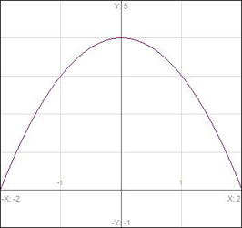
Now let’s examine the parabola ![]() below.
below.

Its derivative ![]() . It also has a critical point at
. It also has a critical point at ![]() . However, it changes from increasing to decreasing at
. However, it changes from increasing to decreasing at ![]() (i.e. its derivative changes from + to –). The point
(i.e. its derivative changes from + to –). The point ![]() in the given interval, is known as a local maximum. Also, in this interval, the function is concave down.
in the given interval, is known as a local maximum. Also, in this interval, the function is concave down.
Some books refer to convexity rather than concavity. Where a function has positive concavity, it has negative convexity, and vice versa. Some books also use the terms a relative maximum and minimum, rather than local maximum and minimum.
There is a third type of critical point, which is any point where a function is not differentiable. Thus, ![]() is a critical point for
is a critical point for ![]() and
and ![]() .
.
For ![]() , use the first derivative test to find:
, use the first derivative test to find:
(A) over which interval the function is increasing and decreasing; and
(B) all local maxima and minima.
(A) ![]() .
. ![]() is increasing whenever the product
is increasing whenever the product ![]() . This occurs when either both terms are positive, or both terms are negative. Therefore,
. This occurs when either both terms are positive, or both terms are negative. Therefore, ![]() . The first condition is met whenever
. The first condition is met whenever ![]() , and the second condition is met whenever
, and the second condition is met whenever ![]() . Another way to write this is that
. Another way to write this is that ![]() is increasing in the ranges
is increasing in the ranges ![]() . It should be obvious (or you can run through the entire argument) that
. It should be obvious (or you can run through the entire argument) that ![]() is decreasing in the open range
is decreasing in the open range ![]() .
.
(B) The local extrema (the local maximum and minimum) are located at the points at which ![]() , which are the points
, which are the points ![]() . In the interval around
. In the interval around ![]() ,
, ![]() changes from positive to negative, which means
changes from positive to negative, which means ![]() is a local maximum. In the interval around
is a local maximum. In the interval around ![]() ,
, ![]() changes from negative to positive, so
changes from negative to positive, so ![]() is a local minimum.
is a local minimum.
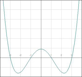
A graph of ![]() in the interval
in the interval ![]() is depicted below.
is depicted below.
![Graph of the interval [5, -5]](http://americanboard.org/Subjects/Images/math/8/images/Math%20Mod%208.3%20Art%20006.JPG)
We can see the local maximum and minimum and ![]() and
and ![]() , respectively. However, it is clear that the local maximum is not the largest value of the function in this interval, and the local minimum is not the smallest value. In the interval
, respectively. However, it is clear that the local maximum is not the largest value of the function in this interval, and the local minimum is not the smallest value. In the interval ![]() , the absolute maximum is at
, the absolute maximum is at ![]() , and the absolute minimum is at
, and the absolute minimum is at ![]() . The first derivative test only identifies relative extrema, that is, the points at which the function shifts direction. Additional analysis is required to determine absolute extrema.
. The first derivative test only identifies relative extrema, that is, the points at which the function shifts direction. Additional analysis is required to determine absolute extrema.
As we have learned, the first derivative of a function can be used to determine concavity (i.e. over what interval the function increases and decreases), and the location of relative extrema. We will call this analysis the first derivative test. We will now show that the second derivative test can be used to determine relative extrema and more.
Let’s look again at our two parabolas, ![]() and
and ![]() . We have already computed their derivatives,
. We have already computed their derivatives, ![]() and
and ![]() . Below,
. Below, ![]() and
and ![]() are sketched again.
are sketched again.
 |
 |
Look carefully at their second derivatives, ![]() and
and ![]() . Note that the second derivative is always positive for
. Note that the second derivative is always positive for ![]() and always negative for
and always negative for ![]() . This is illustrated below by graphs of the derivatives for
. This is illustrated below by graphs of the derivatives for ![]() and
and ![]() :
:
 |
 |
The second derivative is nothing more than the slope of the first derivatives. In the vicinity of a local minimum, the slope of the derivative (i.e. the second derivative) is positive; in the vicinity of a local maximum, the slope of the derivative (i.e. the second derivative) is negative. The same principle holds for any differentiable function where the second derivative exists.
If ![]() is differentiable on an open interval around
is differentiable on an open interval around ![]() , and
, and ![]() exists, then:
exists, then:
(i) ![]() is a local minimum (and
is a local minimum (and ![]() is concave up) if
is concave up) if ![]() and
and ![]() ;
;
(ii) ![]() is a local maximum (and
is a local maximum (and ![]() is concave down) if
is concave down) if ![]() and
and ![]() .
.
At this point, you may be wondering what happens when ![]() . Let’s look at two examples of this situation,
. Let’s look at two examples of this situation, ![]() and
and ![]() .
.
 |
 |
It is easy to show ![]() and
and ![]() . However, the point
. However, the point ![]() is neither a maximum nor a minimum for
is neither a maximum nor a minimum for ![]() , and it is actually a relative minimum for
, and it is actually a relative minimum for ![]() . This tells us that the second derivative test does not always work. If the second derivative is zero, you may need to rely on the first derivative test to determine relative extrema and concavity.
. This tells us that the second derivative test does not always work. If the second derivative is zero, you may need to rely on the first derivative test to determine relative extrema and concavity.
For ![]() , the point at
, the point at ![]() is known as a point of inflection. A point of inflection is any point along a curve at which the concavity changes directions from down to up or from up to down. In other words, the point
is known as a point of inflection. A point of inflection is any point along a curve at which the concavity changes directions from down to up or from up to down. In other words, the point ![]() is a point of inflection if
is a point of inflection if ![]() when
when ![]() and
and ![]() if
if ![]() , or if
, or if ![]() when
when ![]() and
and ![]() if
if ![]() . The function does not have to be differentiable at this point, however. For example, we have seen that the function
. The function does not have to be differentiable at this point, however. For example, we have seen that the function ![]() is not differentiable at
is not differentiable at ![]() . However, you can prove that
. However, you can prove that ![]() satisfies the condition for a point of inflection at
satisfies the condition for a point of inflection at ![]() .
.
With what we know about maxima and minima, we are able to use the first and second derivative tests to solve optimization problems. We will demonstrate this with a couple of classic examples.
A rectangular field which runs to the bank of a straight river needs to be fenced off. There is a total of 2,000 yards of fencing material that can be used. Assuming the river forms one side, what is the maximum area that can be fenced in? Assume the field will have a length ![]() and width
and width ![]() . The total area is
. The total area is ![]() . Let’s assume the river runs along the width. That means that the total amount of fencing material used is
. Let’s assume the river runs along the width. That means that the total amount of fencing material used is ![]() yards. Solving for
yards. Solving for ![]() . We then substitute
. We then substitute ![]() into the equation of the area, and the result is
into the equation of the area, and the result is ![]() . An extreme point occurs where
. An extreme point occurs where ![]() . Therefore, A‘(x) = 2,000 – 4x = 0 or x = 500 yards, y = 2,000 – 1,000 = 1,000 yards, and the area is
. Therefore, A‘(x) = 2,000 – 4x = 0 or x = 500 yards, y = 2,000 – 1,000 = 1,000 yards, and the area is
A = (500)(1,000) = 500,000 square yards.
Is this the maximum or minimum area? The answer can be found by computing ![]() .
.
![]()
Since the second derivative is negative, this area is the maximum.
Let’s try another example. What is the area of the largest rectangle that can be inscribed within the parabola ![]() , as illustrated below? The x-axis defines the length of one side, and two corners lie on the parabola.
, as illustrated below? The x-axis defines the length of one side, and two corners lie on the parabola.
Assume the corners of the rectangle on the x-axis is at ![]() and
and ![]() . Therefore, the rectangle touches the parabola at
. Therefore, the rectangle touches the parabola at ![]() , which is also the length of the rectangle. Therefore,
, which is also the length of the rectangle. Therefore, ![]() . The extreme value for A is
. The extreme value for A is ![]() , or
, or ![]() (we defined
(we defined ![]() as positive). Therefore,
as positive). Therefore, ![]() and
and ![]() . Since
. Since ![]() for
for ![]() , we know this area is the maximum.
, we know this area is the maximum.
Another interesting application of derivatives is Newton’s method for approximating the roots of a function. The roots of a function are those points where the function crosses the x-axis, or where ![]() . They are also known as the zeros of a function. As an example, the function
. They are also known as the zeros of a function. As an example, the function ![]() has four roots:
has four roots: ![]() . Below, we plot
. Below, we plot ![]() in a range where all its roots are visible, as well as the
in a range where all its roots are visible, as well as the
vicinity of the root ![]() .
.
 |
 |
In the second graph, we also include the tangent line at ![]() . Let’s say
. Let’s say ![]() is our initial guess of the root around
is our initial guess of the root around ![]() . That initial guess is not accurate, but notice that the tangent line intersects the x-axis at a point much closer to the root (at about
. That initial guess is not accurate, but notice that the tangent line intersects the x-axis at a point much closer to the root (at about ![]() ). Now, suppose you take the tangent line at
). Now, suppose you take the tangent line at ![]() . That tangent line will intersect the x-axis at a point even closer to the root (at
. That tangent line will intersect the x-axis at a point even closer to the root (at ![]() ). After a few iterations, you will come very close to the actual root.
). After a few iterations, you will come very close to the actual root.
Given ![]() , try
, try ![]() as our initial guess for a root. The tangent line hits the curve at the point
as our initial guess for a root. The tangent line hits the curve at the point ![]() , has a slope
, has a slope ![]() , and we’ll say it crosses the x-axis at
, and we’ll say it crosses the x-axis at ![]() . With these two points and the slope, we can solve for
. With these two points and the slope, we can solve for ![]() .
.
![]()
Therefore, ![]() . With
. With ![]() as our new guess, we can repeat the process.
as our new guess, we can repeat the process.
It should be clear that, for the ![]() iteration:
iteration:
![]()
Let’s try an example. Assuming an initial guess of ![]() , use Newton’s method to approximate
, use Newton’s method to approximate ![]() .
.
The value ![]() is the positive root of the equation
is the positive root of the equation ![]() . Since
. Since ![]() , we have
, we have ![]() . We start with
. We start with ![]() . You may want to use a calculator for these calculations.
. You may want to use a calculator for these calculations.
The value ![]() is as close to
is as close to ![]() as a 10-digit calculator can calculate.
as a 10-digit calculator can calculate.