Differential Equations, Sequences, and Series

What is a differential equation?

A differential equation is an equation that contains derivatives. The order of a differential equation is the order of the highest ordered derivative in the equation. Thus,  is a first-order differential equation, while  is a second-order differential equation. A thorough study of differential equations is typically reserved for advanced calculus. This lesson examines elementary differential equations of the forms and , where  is a constant.

Suppose  represents a quantity such as a population of bacteria, the volume of a dye used in a medical analysis, the mass of a decaying radioactive substance, the future value of a compounded investment, etc. Then, the quantity  represents the growth of . In these and other applications, the relative rate of growth is proportional to its quantity; that is, , where  is the constant rate of increase  or decrease  in the quantity. Rewriting the equation as , we find , or . Integrating both sides, we get . Therefore, . This equation has the solution  where  is a positive constant. 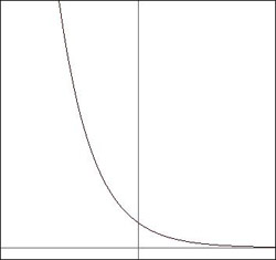Therefore,  where  can be any real number. This equation describes exponential growth and decay, which is represented graphically below for  and  respectively.

There are an infinite number of solutions to this differential equation, as the choices for  and  are infinite. Typical physical problems, however, have a single solution. This is rectified by specifying initial conditions, such as  where  and  are given or measured.

Differential Equations, Sequences, and Series

Let’s try some examples. The rate of growth of a bacteria culture is proportional to its population. Initially, the population is 10,000, but it increases to 25,000 after 10 days. What is the size of the population after 20 days?

This is an exponential growth problem of the form , where  is the population after t  days, and . The general solution is . At this point, we have an equation for the population with two unknowns. To find a unique solution, we are given two initial conditions: (i) , and (ii) . Initial condition (i) gives us  or  Initial condition (ii) gives us:  Therefore,  Taking the natural log of both sides. , so . Therefore,

 is the unique solution for the population at any time t. After 20 days,

Newton’s law of cooling says that the rate of change in temperature  of an object is proportional to  the temperature difference between the object and its surroundings. If the constant of proportionality is , and the initial temperature is  (A) find an expression for  in terms of  and , and (B) in terms of , how much time does it take for the temperature difference to be cut in half?

(A) Over time, the temperature of the object approaches the temperature of the surroundings; therefore, the difference decreases over time, so this is an example of exponential decay. We note  for , so . Our initial  condition is  so our expression for  is

.

(B) We want to find the time  for which . We find , so . Therefore,

Differential Equations, Sequences, and Series

The next differential equation we examine is the form or , where  is a constant. As a guess, assume a solution . We find:

,

or

,

which satisfies the differential equation when . Although we chose a cosine function, this also applies to a sine function. The  variable allows for the shift from cosine to sine. Since the cosine function repeats itself over time, this differential equation describes periodic motion or oscillations. We are typically interested in periodic and bounded motion, known as harmonic motion.

The -term is known as the angular frequency, measured in radian/sec. The term  is called the phase of motion, and  is the phase constant. If we imagine an object moving in a circle of radius  about the origin,  is the angular displacement from the x-axis at , and  is the angular speed of the object.

Here is an example. Newton’s second law of classical mechanics states that a force  acting on a constant mass  is proportional to the acceleration  of the mass, . Previously, we learned that acceleration is the second derivative of the position function; that is,  (assuming we restrict motion to the x-direction). We also learned of Hooke’s law, which states that the force exerted by a spring that is displaced a distance  from its natural position is , where  is a constant. Suppose a mass   attached to the end of a massless spring of spring-constant  is placed on a frictionless surface and is initially stretched a distance  from its natural position. (A) Show that the behavior of the spring-mass system is described by harmonic motion, and (B) find the angular frequency in terms of  and .

(A) Setting both force equations equal to one another, we find , or  Since  and  are both positive constants, the ratio  is positive. This is in the form , and is therefore an equation for harmonic motion.

(B) From the equation , we know 

What are sequences and series?

A sequence is a function whose domain is the set of positive integers. Recall that the domain of a function  is the set of all possible values of . For example, the sequence  has the reciprocals of all positive integers as its elements.

If  is a sequence, then  is known as a series. Each  is a term of the series. Of special interest is an infinite series, where the number of terms is infinite. A geometric series is an infinite series where consecutive terms differ by the same ratio; the simplest form is , where  is constant. A power series is of the form  (specifically, a “power series in ”), and it will be given special treatment in this module.

Sequences and series can be convergent or divergent. The sequence  is convergent if  for some finite value . If  or cannot be defined (for example, if the sequence eventually settles into a pattern of oscillation between two distinct values) , the sequence is divergent. Likewise, an infinite series is convergent if the sum approaches a finite value, and is divergent if the sum blows up to 
or cannot be defined. It is easily proven that, if an infinite series  is convergent, then  Are the following sequences convergent or divergent?

(A)  so we use L’Hôpital’s rule.

The sequence converges to 

(B)  so the sequence is divergent.

(C) The sequence forever alternates between  and , so it is divergent.

For what values of r is the infinite geometric series  convergent?

The series is convergent if and only if  For , the limit blows up to . For  the limit alternates between  For , the limit approaches . For , the limit alternates between . Since none of these limits approach 0, the series is divergent for  However, for the values , we can express  as a fraction , where  and . Therefore,  since  Therefore, the series is convergent for .

Differential Equations, Sequences, and Series

If an infinite series converges, there may or may not be techniques for calculating the exact sum. For the case of the example, we will later show that the sum converges to  for . Furthermore, if  and  converge, then  converges, and  converges as well.

There are several tests to determine whether an infinite series of the form  is convergent or divergent. For the case of an infinite series consisting only of non-negative terms, we have three tests at our disposal: the comparison test, the limit comparison test, and the integral test.

An example of each convergence test should help illustrate their power.

For the series , , use the integral test to determine the values of  for which the series converges and diverges.

First, we note that  is continuous, positive, and decreasing for . For , we find

Therefore, the series diverges for . For ,

Therefore, the series converges for . Finally, for ,

Therefore, the series diverges for . If we put it all together, we find that  diverges for  and converges for . The series for  is known as the harmonic series.

Given the above conclusion that the harmonic series diverges, use the comparison test to determine whether  converges or diverges.

For , , so . Since we know the harmonic series diverges, the comparison test tells us that  diverges as well.

Solve the example using the limit comparison test, again using the harmonic series for comparison. Let  and . We find,

Therefore, part (iii) of the limit comparison test tells us that  diverges.

Differential Equations, Sequences, and Series

The study of infinite series is not restricted to positive terms. One common infinite series with both positive and negative terms is known as an alternating series. It has the form . The following theorem is a test of convergence specifically for the alternating series.

Determine if the alternating series  is convergent or divergent.

Note that this series has nearly the same terms as the harmonic series (which is divergent), but the signs alternate.  and , and  for , so the first condition applies. We find , so this alternating series is convergent. The above series  is convergent, but the harmonic series  is divergent. An infinite series like this is said to be conditionally convergent if  is convergent but  is divergent. If both series are convergent, then  is said to be absolutely convergent. If a series is absolutely convergent, it is also convergent. With this understanding of absolute convergence, we introduce two new tests for absolute convergence: the ratio test and the root test.

Here are a few more examples.

Using the ratio test, determine whether  converges or diverges.

We find .

Therefore, the series is convergent.

Using the root test, determine whether  converges or diverges.

. Applying L’Hôpital’s rule,
. Therefore, the root test is inconclusive.

We previously defined a power series in  as a series of the form

 . A power series in  is of the form

 where  is a real number. However, we can easily convert this to the first power series by setting  and defining a power series in  Therefore, we restrict our analysis to the first form of power series for the following section.

For the power series , we define the radius of convergence as a number  such that s converges if  and diverges if . At  the series may either converge or diverge. If  converges only when , then If  converges for all real values of  then 

The set of values of  for which  is convergent is known as the interval of convergence. If  is known, the interval of convergence can be determined. If , the interval of convergence is 0. If  the interval of convergence is . Finally, if  it is necessary to check . Depending on the convergence or divergence at these two points, the interval of convergence is 

We can determine the radius of convergence by applying either the ratio test or root test to the  portion of the series.

For the power series , what are the radius of convergence and interval of convergence?

Apply the ratio test. 

The ratio test tells us that if , then the series is convergent, and if , then the test is inconclusive. So we know that if |x| < 1, then the series is convergent, and if |x| = 1, the series may or may not be convergent. We will need to check x = 1 and x= –1 individually. Either way, .

Now we check  and . At , the series is , which converges by the alternating series theorem. At , the series is , which converges, as we saw in the example. Therefore, the interval of convergence is .

If a power series has an interval of convergence, we can define a function  to describe the power series for each  in that interval, . In some cases,  is a familiar function and is easy to derive. For example, we can derive  for the simple geometric series . In the example, we showed that  exists in the interval of convergence of . We compute . Since s is not infinite in the interval of convergence, we can subtract the second term from the first. Note that all terms except 1 are eliminated.

So, . Therefore, , or  for . With this, we can define other functions. For example, , and , where  still holds.

Differential Equations, Sequences, and Series

Since a power series can be expressed as a function  within its interval of convergence,  exist within the same interval. For the differentiation and integration of power series, we perform the appropriate calculation—term by term. If the power series has a radius of convergence , then for :

(i) is continuous.

(ii) exists.

(iii) exists.

Thus differentiating or integrating a power series forms a new series with the same radius of convergence. From this, we can derive other interesting functions expressed as infinite series.

From , for , find the power series expression for  and  for .

By differentiating, we find 

By integrating, we find . By substituting , we find , or . Therefore, .

Prove that 

First, we need to find the interval of convergence. By applying the ratio test, we find that . Thus the radius of convergence is , and the interval of convergence is . Next, take the derivative of both sides of 

, where we substituted . Note that we find . The solution for this differential equation is . At , , so . This completes the proof.

Since the function is continuous and differentiable within the same interval of convergence, it follows that higher order derivatives exist on the same interval. Since the series is infinite, the function  is infinitely differentiable on the interval. Taking the first few derivatives of the power series, we find

,

,

.

At this point, note the following patterns for .

Differential Equations, Sequences, and Series

In general, we can define the coefficients  as , and the power series in x can be rewritten as

.

The above series is known as the Maclaurin series. Generally, we can define the power series in ,

and take the same steps to show

This series is known as the Taylor series of  at . While the Maclaurin series has an interval of convergence , the Taylor series has an interval of convergence . A series that is taken to the  order rather than to  is called an  degree Taylor polynomial. In calculations, we typically use Taylor polynomials to attain a desired degree of accuracy.

Suppose we define an  degree Taylor polynomial as . We call the difference between the function  and the Taylor polynomial the remainder term  in the interval of convergence. Therefore, . It can be shown that , where each  is between  and .

Find the Maclaurin series expansion for .

Set . All higher order derivatives , so . Therefore,

Note that this was proven in the example to be true for all . Strictly speaking, this is not a formal proof that  has a series expansion. It simply shows that if  has a Maclaurin series expansion, then this series must be it.

Find the Taylor series expansion for  at .

The Taylor expansion is therefore

Approximate the value of  using the first 6 terms of the Taylor expansion. Compute the value using a ten-digit calculator and determine why both answers are exactly the same.

In radians, . Using the above formula for  at ,

Using a ten-digit calculator, you should find the same value. The reason for this high degree of accuracy can be found in the remainder term. The error introduced by using the first six terms is , which is

This shows that the above result should be accurate to  decimal places, which is better than a ten-digit calculator.

Further Reading in Calculus

Calculus (Ron Larson and Robert P. Hostetler): Houghton Mifflin, 2003.

Calculus Demystified: A Self-teaching Guide (Steven G. Kranz): McGraw-Hill, 2003.

Calculus Made Easy: Being a Very-Simplest Introduction to Those Beautiful Methods of Reckoning Which Are Generally Called by the Terrifying Names of the Differential Calculus (Silvanus Philips Thompson and Martin Gardner): St. Martin’s Press, 1998.

How to Ace Calculus: The Streetwise Guide and How to Ace the Rest of Calculus: The Streetwise Guide. (Colin Adams, et. al.): Henry Holt and Company, 1998.

The Complete Idiot’s Guide to Calculus (W. Michael Kelley): Alpha Books, 2002.

Don’t forget to test your knowledge with the Calculus Chapter Quiz;